Geology 319 Structural Geology: The Architecture of Earth’s Continental Crust

Study Guide :: Unit 4

Faults

Overview

In Unit 4 you will learn about faults. After studying the classification of faults in Lesson 1, Lesson 2 will cover how stress controls which kind of fault will form. Lessons 3, 4, and 5 discuss specific types of faults in more detail: Lesson 3 covers thrust faults, Lesson 4 covers normal faults, and Lesson 5 covers strike-slip faults. In Lesson 6 you will learn how faults affect topography and control scenery. Lesson 7 compares brittle and ductile faulting, and examines the conditions necessary for a fault to generate earthquakes, while Lesson 8 surveys rocks and structures that are found in fault zones.

Objectives

After studying this unit, you should be able to

1. sketch all the major fault types as cross-sections and block diagrams.
2. describe the stress regime under which each type of fault occurs.
3. explain the difference between brittle and ductile faulting, describe the fault rocks associated with each, and detail how one can determine the direction and sense of slip.
4. describe the process that generates earthquakes.
5. describe the ways in which faults affect topography.
6. describe the structures associated with specific types of faults.
7. determine fault type from information on a geological map.

Lesson 1: Classifying Faults

Faults are fractures along which rocks have been offset. A fault zone is a region where many faults occur near each other. In an area in which the rock is weak and broken up, an obvious fracture may not be evident, yet displacement has obviously occurred, so this is also considered a fault zone.

Faults are a way by which rocks redistribute stress. For example, they are an important way that tectonic forces are accommodated in orogens, allowing the rocks in orogens to shorten in response to compression. Faults can also be important economically: when faults act as conduits for the flow of groundwater, the rocks in fault zones can be altered either by partial solution or by precipitation of some of the chemical elements being carried by the groundwater. In the latter case, gold and some copper deposits can form in fault zones.

There are two main ways to classify faults: 1) according to the kind of deformation that occurs (Fig. 4.1) or 2) according to the direction of displacement or slip. When classified according to deformation, faults may be ductile (also referred to as ductile shear zones), brittle, or both (brittle-ductile shear zones).

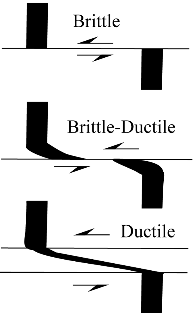
Figure 4.1. Classification of faults according to style of deformation

The second way of categorizing faults is with reference to the direction of displacement or slip. Slip is described in terms of relative movement, because it is usually not possible to identify the actual motion that took place. For example, it is not possible to determine whether a slip occurred by movement of the rocks on one side of the fault while the other remained stationary, or (as is more likely) by movement on both sides of the fault.

The system for classifying faults according to their main component of slip is summarized in Figure 4.2. Strike-slip faults have horizontal movement along the strike of the fault surface. They are further classified as either sinistral (left-handed), or dextral (right-handed) depending on the direction of separation with respect to a chosen point of reference. (Fig. 4.2 explains how this works.)

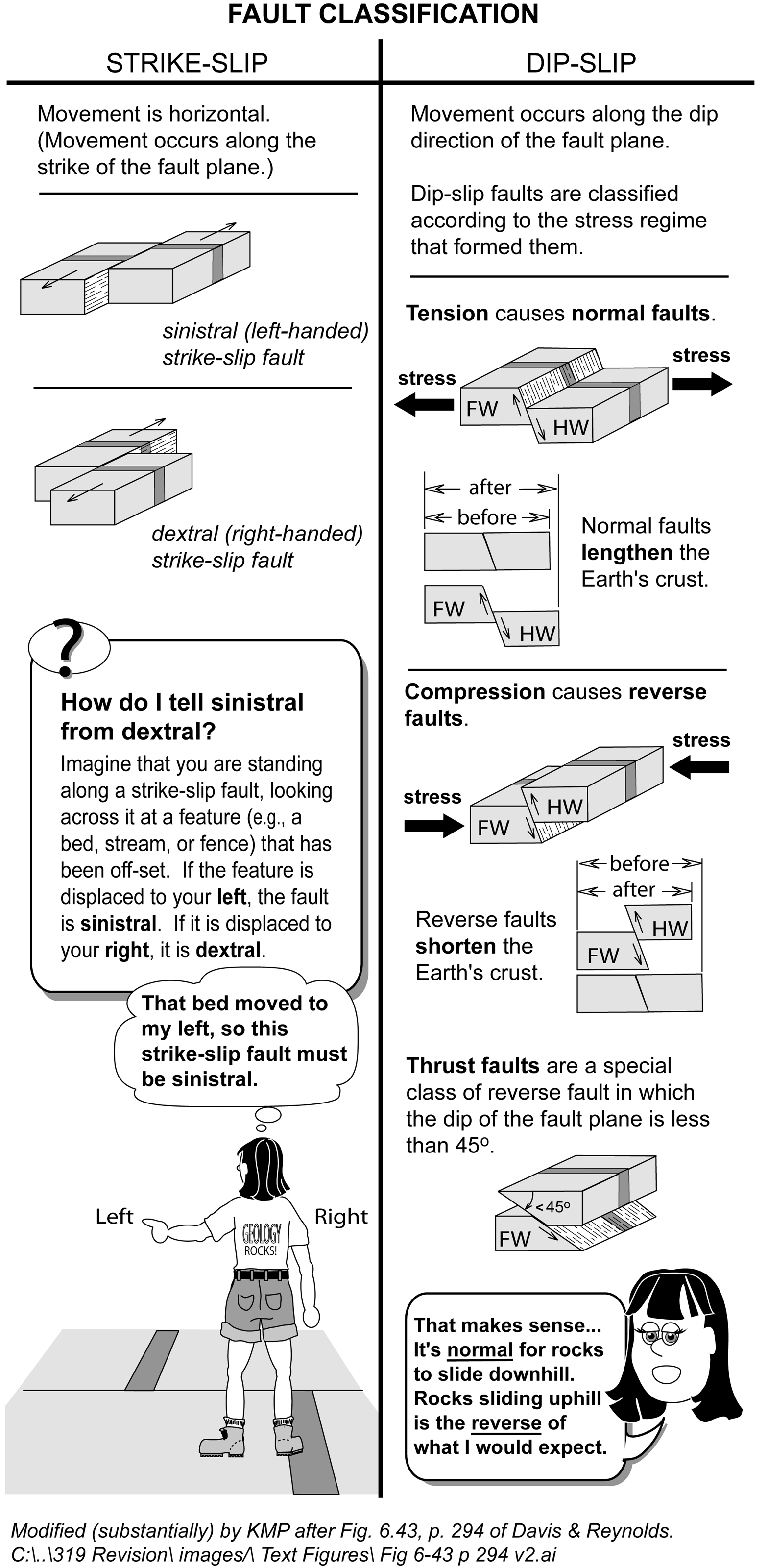
Figure 4.2. Fault classification

Dip-slip faults have movement either up or down the fault surface. They are often described in terms of the relative motion of the hanging wall and footwall blocks of the fault. The footwall is the block on the underside of the fault, and the hanging wall is the block above the fault. To remember the difference, imagine that you were in a mine drift cut through the fault. In this context, you could “hang” a lantern on the hanging wall block, because it would be the roof of the drift. You would be standing on the footwall block. Some students also find it convenient to simply draw a point on the fault (e.g., P in Fig. 4.3). The block directly above P is the hanging wall, and the block directly below P is the footwall.

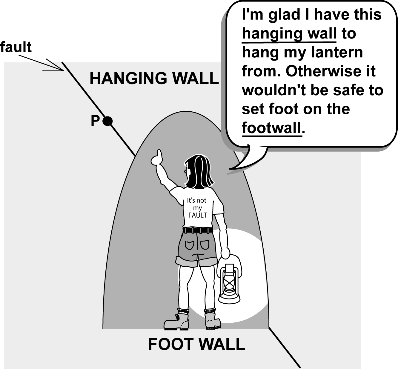
Figure 4.3. Tricks for determining the hanging wall and footwall of a fault

Normal faults are dip-slip faults that result in extension of rocks. For a normal fault, the hanging wall moves down with respect to the footwall. Reverse faults are dip-slip faults that cause shortening of rocks. The hanging wall moves up relative to the footwall on reverse faults. Thrust faults are a special case of reverse faults in which the fault surface is at a low angle to the horizontal. Thrust faults are particularly important in orogens.

Nature never operates as tidily as these classification systems, of course. As such, faults frequently have some combination of dip slip and strike slip, even if one component is much smaller than the other. As an operational definition, geology uses a 5:1 ratio as a cut-off point. Therefore,

• if the amount of strike slip is five or more times greater than the dip-slip component, the fault is considered a strike-slip fault; and
• if the amount of dip slip is five or more times greater than the amount of strike slip, then the fault is considered a dip-slip fault.

The intermediate cases, in which no one component is five times larger than the other, are called oblique-slip faults. Any kind of strike-slip fault may be combined with any kind of dip-slip fault, resulting in four kinds of oblique-slip faults:

• sinistral normal,
• sinistral reverse,
• dextral normal, or
• dextral reverse.

Two examples of oblique-slip faults are shown in Figure 6.42C (Davis, Reynolds, & Kluth, p. 273).

In addition to dip- and strike-slip, rotation can occur on a fault surface (Fig. 6.42D, Davis, Reynolds, & Kluth, p. 273). This can happen in a number of geological settings (e.g., along faults produced over rising plutons), but it happens most commonly at the ends of dip-slip faults, where the amount of slip is dying out. In such a case, the main part of the fault is still a dip-slip structure—the local rotation is merely a minor modification of the overall slip.

Reading Assignment

• Read Davis, Reynolds, & Kluth: “The Naming and Classification of Faults” (pp. 272-277)

Study Questions

1. How do faults differ from joints or fractures?
2. Why is it important to distinguish between separation and slip?

Lesson 2: How Stress Controls the Shape of Faults

Anderson (1951) came to the surprising conclusion that only normal folds, thrust folds, and strike-slip folds should be able to form at or near the Earth's surface. This means that reverse faults should not be able to form near Earth's surface. His work also provides an explanation for why, on average, strike-slip faults tend to be vertical, thrust faults tend to dip at 30°, and normal faults tend to dip at 60°.

Anderson began with the observation that at the interface between the atmosphere and the Earth's surface, there is no shear stress. Because principal stress directions are directions where shear stress is zero (by definition), the two-dimensional plane at Earth's surface must contain two of the three principal stresses. The third will always be oriented perpendicular to Earth's surface.

2.1. The Sandbox Model

The other piece of the puzzle is that the angle of internal friction (ϕ) averages 30°, regardless of rock type. The angle of internal friction reflects the ratio of normal stress to shear stress that will cause a rock to break, or fail. It describes the amount of force required to overcome the force of friction of a material sliding over itself. The sandbox experiment provides a good model. The first step in the sandbox experiment is constructing the failure envelope for sand: the experimenters must determine what amount of shear force is required to cause one sand-filled frame to slip over a second sand-filled frame (Fig. 6.78, Davis, Reynolds, & Kluth, p. 294). They must do so for varying amounts of normal force. The normal force is provided by rocks of known mass stacked on top of the experimental apparatus. An experimenter provides the shear force by pulling on the upper sand-filled frame. The experimenters plot the normal and shear stresses at which the upper frame begins to move, and fit a line to their data (Fig. 6.79, Davis, Reynolds, & Kluth, p. 294). This line is the failure envelope. The dip angle of the failure envelope is the angle of internal friction. As expected, for unconsolidated sand, ϕ = 30°.

The angle of internal friction is important, because the fault that forms when a material fails will be oriented at an angle to the maximum principle stress. That angle is ϕ. Returning to the sandbox experiment (Fig. 6.80, Davis, Reynolds, & Kluth, p. 295), movement of the partition to the right sets up two different stress regimes. On the left-hand side, this movement creates a maximum principal stress that is vertical (90°), because the partition no longer supports the sand from the side. Normal faults form with dip angles of 60° (i.e., 30° away from vertical). On the right-hand side of the box, movement of the partition compresses the sand, so the maximum principal stress is horizontal. Here, thrust faults form with dip angles of 30°.

Reading Assignment

• Read Davis, Reynolds, & Kluth: “Hubbert's Sandbox Illustration of Coulomb Theory” up to “Mohr Diagram Portrayal of the Sandbox Experiment” (pp. 294-296)

2.2. Beyond the Sandbox

In foliated rocks or in rocks where there are pre-existing fractures, faults may not conform to classic sandbox behaviour. It takes less stress to reactivate pre-existing fractures than it does to break a rock in the first place. Furthermore, fractures may be reactivated that are oriented as much as 65° away from the direction of greatest principal stress. With foliation, if the foliation is at a high angle to the direction of greatest principal stress, then faults will develop that are consistent with theory. However, if foliation is parallel to σ₁, a fault that develops will be oriented at a much smaller angle to σ₁ (e.g., 10° or 20°). If the foliation is oriented between 25° and 45° to σ₁, the fault will have the same orientation as the foliation.

Reading Assignment

• Read Davis, Reynolds, & Kluth: “Faulting of Anisotropic Rocks” (pp. 296-297)

2.3. Reverse Faults

Reverse faults result in crustal shortening; they usually have dips of 60° or greater; and they do not conform to the sandbox model discussed above. One explanation for their formation is fault reactivation. The reverse fault may have formed as a normal fault to begin with, but a change in the stress regime may have caused a second slip, this time as a reverse fault (Fig. 6.89, Davis, Reynolds, & Kluth, p. 302). Another explanation for a reverse fault is that the directions of principal stress may not be vertical and horizontal at depth. In fact, a curved stress trajectory may develop, leading to curving faults (Fig 6.92, Davis, Reynolds, & Kluth, p. 303). One part of the curved fault may be a thrust fault, but the slope of the curve may steepen into a reverse fault.

Reading Assignment

• Read Davis, Reynolds, & Kluth: “The Problem of Reverse Faults” (pp. 301-303)

Study Questions

1. Normal faults form when the Earth's surface is in tension. Why is the maximum principal stress for a normal fault not horizontal, in the direction of the tension?
2. True or false? A reverse fault can occur at Earth's surface.

Lesson 3: Thrust Faults

Thrust faulting is the most important way in which rocks of geosynclines become shortened and uplifted into mountainous orogens. Thrust faults that form in relatively shallow rocks are brittle structures, but thrust faults are ductile at depths greater than approximately 5-10 km, depending partly on the local geothermal gradient. Many brittle thrust faults are exposed in young orogens such as the eastern part of the North American Cordillera. Displacements differ from one thrust fault to another. In several orogens, displacements with more than 100 km of horizontal shortening occur, while hundreds of orogens with displacements of 10-50 km are known.

Thrust faults display a variety of common geometric features. Figure 4.4 shows a series of cross-sections displaying increasingly complex structures:

• (a) shows a single, straight, gently dipping thrust, in which neither the hanging wall block (HWB) nor the footwall block (FWB) has been distorted. The leading edge of any particular rock formation in the hanging wall block is called the toe of the fault. The hanging wall block is commonly referred to as the thrust sheet.
• (b), (c), and (d) demonstrate increasing folding in both the HWB and FWB. Note that the HWB and FWB need not be distorted in identical ways. Folds may be overturned and the strata turned locally upside down, especially near the fault.
• In (e), a series of parallel thrusts have resulted in an imbricate fault system with three thrust sheets. Each of the two lower thrusts sheets is the hanging wall block of the fault below, as well as the footwall block of the fault above. Note that the thrust sheets could be deformed as in Figure 4.4(b-d).
• Thrust faults curved concave upwards are called listric thrusts, as in (f). Here, the HWB is folded, but the FWB is not. Some of the folding of the HWB is due to rotation of the beds caused by the curvature of the fault.
• (g) demonstrates listric sole thrust with several branching faults or splay faults of smaller displacement, forming an imbricate stack of thrust sheets. The total fault displacement is the sum of the individual displacements.
• Thrusts can be folded. In (h), a listric stack of splay faults branches off a lower sole thrust, with variable degrees of folding. This is a fairly common situation that indicates that folding and thrusting occurred over the same time span: the sole thrust formed first, then the splays, while the folds developed progressively throughout. These are common structures in the foothills of western Alberta. They act as petroleum traps in some of the western oilfields.

Reading Assignment

• Read Davis, Reynolds, & Kluth: “Thrust Fault Systems” up to “The Mechanical Paradox of Overthrusting” (pp. 305-309)

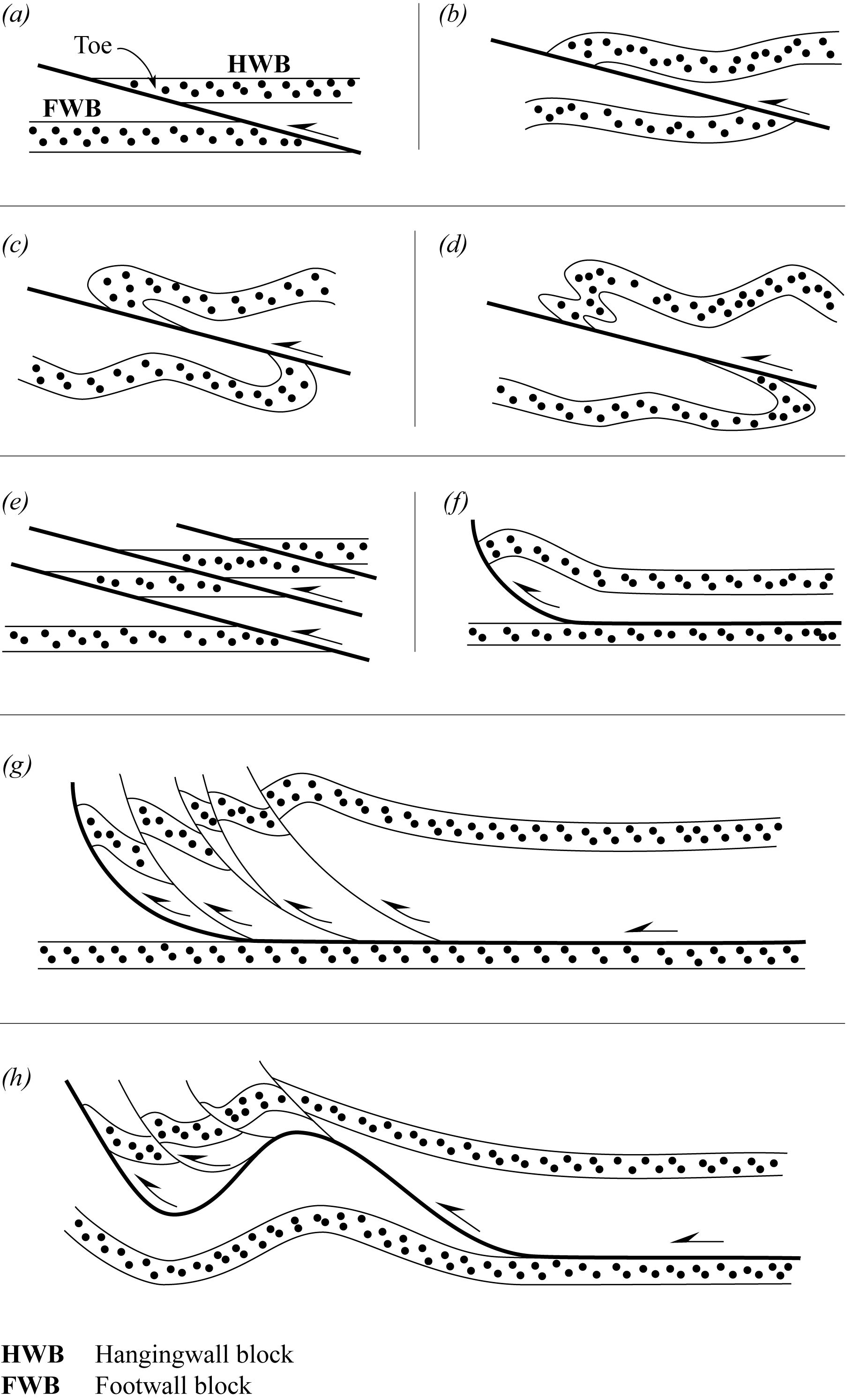
Figure 4.4. Cross-sections through thrust faults

Figure 4.5 (below) shows what happens when a thrust fault cuts through beds of different strengths. In weaker, or incompetent, beds (such as shale), the dip of the fault tends to be shallow. In stronger, or competent, beds (such as sandstone, limestone, or lavas), the dip is steeper. The strong beds are textured in all parts of Figure 4.5.

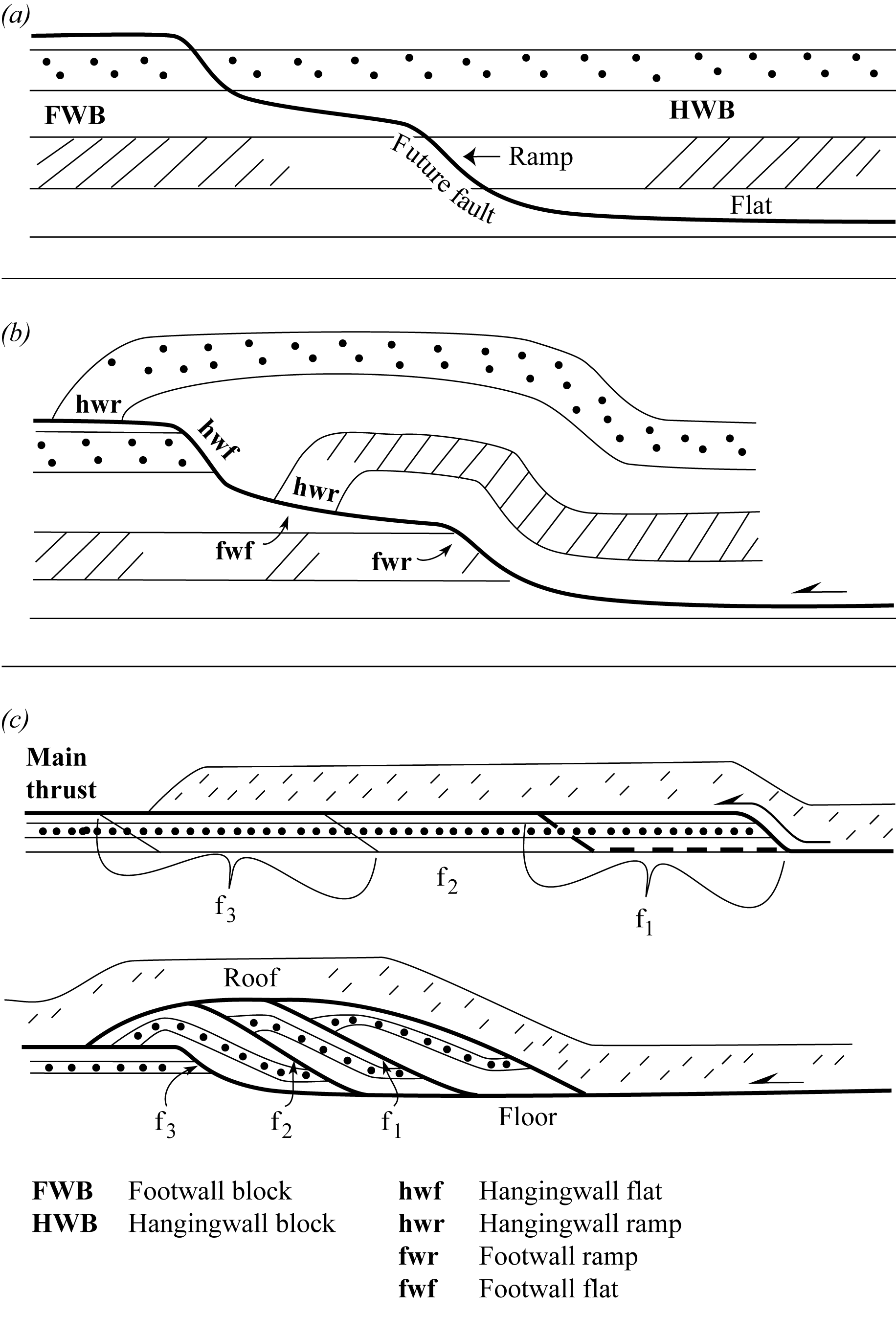
Figure 4.5. Thrust faults with changing dip

• (a) indicates the initial stratigraphic situation and the position of the future fault, with steps or ramps where the fault will cut the stronger beds and more gently dipping flats where it will cut the shale.
• (b): After fault displacement of the HWB (the FWB may or may not be similarly displaced), folds have developed over the steps as the thrust sheet moves, but contact is maintained with the FWB below. Those portions of the HWB originally at a ramp position are called hanging wall ramps (hwr), even though they might have been displaced to lie on the footwall flat (fwf).
• (c) indicates the development of a duplex structure. In the upper part of (c), the main thrust fault (with a step) has brought up a thrust sheet from some depth below the FWB. After some movement on this main thrust fault, it jams up or locks in the vicinity of the step. A new segment develops, (f₁: dashed line) which also forms a step, and it too jams after it slips. This leads to the formation of f₂, which slips and jams, leading to the formation of f₃. The final structure appears in the lower part of (c). The lower-most thrust fault of this duplex structure is the sole or floor thrust, while the upper-most fault is the roof thrust. The imbricate thrust slices are commonly called horses. In this case, the roof thrust is the main thrust, and it has undergone the most movement.

Figure 4.6 shows a single folded thrust. For clarity, only one offset and folded bed is shown. The footwall cutoff (fwco) is the line of intersection between the fault and the base of the sliced bed that forms the footwall. The hanging wall cutoff (hwco) is the line of intersection between the fault and the base of the sliced bed that forms the hanging wall. The distance along the fault surface between these two cutoff lines is the slip undergone by the fault. The short, thin lines on the fault surface indicate the local slip direction. In real rocks, these lines might be represented by structures such as slickenside striations.

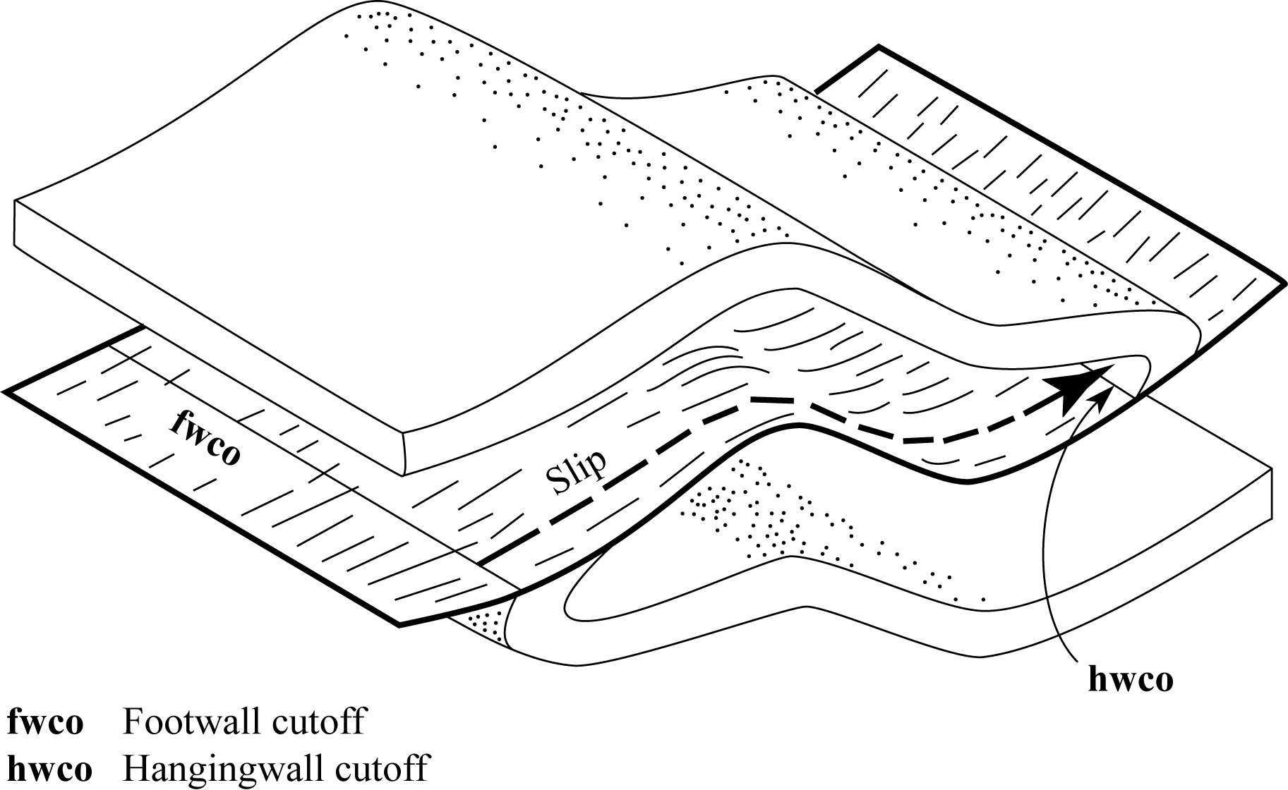
Figure 4.6. Single folded thrust

A few other concepts and synonyms are useful in describing thrust faults. Thrust sheets or thrust plates that have travelled a considerable distance (say, more than 5 km) are commonly called allochthonous blocks or nappes. The footwall blocks to allochthonous thrust sheets are commonly called autochthonous blocks. These terms presuppose that the hanging wall block has moved while the footwall block has remained stationary, a concept called overthrusting (as opposed to underthrusting). Although both blocks do, in fact, move, while hanging wall blocks have been elevated, the footwall blocks may not move down an equal amount (it is harder to push a body of rock into the earth than to push it up; on the way up, it only has its own weight to overcome). As a result, the footwall block is commonly less deformed than the hanging wall block.

A major fault (with or without splays above it) is a sole fault, but it also may be called a decollement, or a detachment fault.

Reading Assignment

• Read Davis, Reynolds, & Kluth: “Ramp-Flat Geometry and Kinematics” up to “The Sequence of Thrusting in Duplexes” (pp. 313-319)
• Read Davis, Reynolds, & Kluth: “The Mechanical Paradox of Overthrusting” up to “Ramp-Flat Geometry and Kinematics” (pp. 309-313)

Study Questions

1. What effect do thrust faults have on the Earth's crust?
2. In the Canadian Rockies, strongly folded and faulted rocks sit above older basement rocks that display none of this deformation. Explain this.
3. Why do some thrust faults form a series of steps and ramps?
4. Hubert and Rubey (1959) calculated that the amount of force required to move thrust sheets the size of those found in the Canadian Rockies would crush the rocks before they ever budged. Yet these thrust sheets exist. How can this paradox be resolved?

Lesson 4: Normal Faults

Normal faults have almost as much overall geotectonic significance as thrust faults. The displacements of the largest normal faults, however, are only about 1/5 that of the largest thrust faults. The largest normal faults have displacements of about 20 km (e.g., some of the low-angle faults in the American southwest Basin and Range Province); they are as rare as thrust faults with 100 km displacement.

Normal faulting can lead to the production of horst and graben structure (Fig. 4.7, below; Fig. 6.122,Davis, Reynolds, & Kluth, p. 323). Down-dropped blocks, called graben, are bounded on both sides by one or more oppositely dipping faults. The higher, possibly uplifted, blocks between are called horsts. Graben commonly become sedimentary basins, and may even contain volcanic material. Grabens are also important where rifts are developing. They can grow to become arms of oceans, as in the Red Sea.

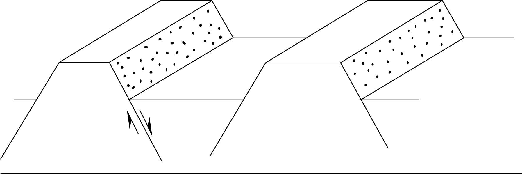
Figure 4.7. Horst and graben structure.

From the standpoint of creating sedimentary basins, even more important is the situation where all the normal faults dip in the same direction (Fig. 6.134, Davis, Reynolds, & Kluth, p. 331). In cases like this, the faults are listric and the down-thrown side rotates, forming a basin that is triangular when viewed in cross-section, although appearing elongate on the earth's surface. Called half-graben, such basins are bounded by one or more faults on one side only. Note in Figure 6.134 the way Late Cenozoic sediments progressively fill the half-graben as faulting continues. Sediments eventually bury what was originally higher ground. Sedimentary basins formed by half-graben are among the lowest spots on Earth's continents (e.g., Death Valley, California).

Reading Assignment

• Read Davis, Reynolds, & Kluth: “Normal Faulting” (pp. 321-333)

Study Questions

1. What effect do normal faults have on the Earth's crust?
2. Why did it take geologists so long to recognize the existence of low-angle normal faults?
3. How do low-angle normal faults form?

Lesson 5: Strike-slip Faults

The largest strike-slip faults active today are all transform faults. These include the Alpine Fault in New Zealand, the San Andreas Fault in California, and the Dead Sea Fault, along which flows the Jordan River between Israel and Jordan. Strike-slip faults have undergone up to five times more slippage than even the largest displacements on thrust faults, which, in turn, are five times larger than the biggest normal faults. For example, the Alpine Fault has undergone nearly 500 km of slip; some estimates of slip on the San Andreas suggest nearly 600 km.

A very important feature of strike-slip faults is that they curve (Figs. 6.146 and 6.147, Davis, Reynolds, & Kluth, p. 339). Where bends or jogs form, parts of the fold that collide with each other are called transpressional bends or restraining bends. There are also bends that move away from each other, called transtensional bends, or releasing bends. Along large strike-slip faults, transtensional bends are especially important, because they commonly form actively growing holes in Earth's crust. These holes become filled with sediment shed off adjacent higher areas (or partly with volcanic rock). Such places are found among those continental regions that have the lowest elevations (e.g., the Dead Sea region).

Reading Assignment

• Read Davis, Reynolds, & Kluth: “Strike-Slip Faulting” (pp. 334-343)

Study Questions

1. True or False? The San Andreas Fault is the boundary between the North American and Pacific tectonic plates.
2. What happens at the bends and jogs along strike-slip faults?

Lesson 6: Faults and Topography

Topographic variation is caused by a number of interacting phenomena: volcanism, sedimentation, uplift of fault blocks, depression of other fault blocks, variation in erosional resistance of various rock types, and the existence of zones of weakness, such as faults, joints, bed contacts, and cleavage. In the global view, the effect of faulting is, however, probably the single most important of these.

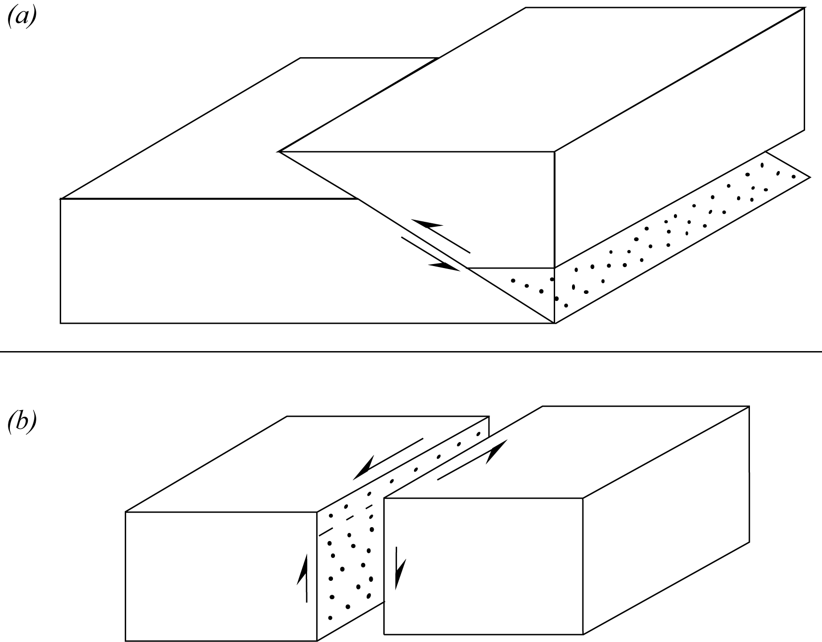
Figure 4.8. Topography caused by thrust faults (a) and strike-slip faults with a dip-slip component (b).

The creation of topographically low places, resulting in sedimentary basins, has already been discussed for normal faults (horst and graben structure, Fig. 4.7) and strike-slip faults (transtensional basins, Figs 6.146 and 6.147, Davis, Reynolds, & Kluth, p. 339). Basins also form on the footwall sides of some thrust faults. Figure 4.8 (above) shows the topography that would develop from a thrust fault (a), and from a left-hand strike-slip fault, with some vertical component of movement (b), in the absence of erosion. Note, however, that erosion does modify these structures, either as they form, or afterwards. The ultimate effect of erosion depends greatly on the relative ease with which the various faulted rocks undergo erosion.

Figure 4.9 shows a common sequence of erosional topographic development, where a resistant (strong) rock overlies a less-resistant (weak) rock. The diagram shows a normal fault, but any other fault with at least some vertical offset will result in a similar situation. Initially, the fault surface itself might form the topographically steeper slope (perhaps a cliff) called a fault scarp. After erosion removes the fault scarp proper, a fault-line scarp remains. The fault line is the trace of the fault on the ground surface. At this stage, it will lie at or near the base of the scarp. The rock near the fault line might be more easily eroded than the adjacent rock, so it might form a fault-line valley where the upthrown side is topographically higher than the downthrown side. Thus, topography mimics structure. Both Figure 4.9 (a) and (b) represent first-order topography.

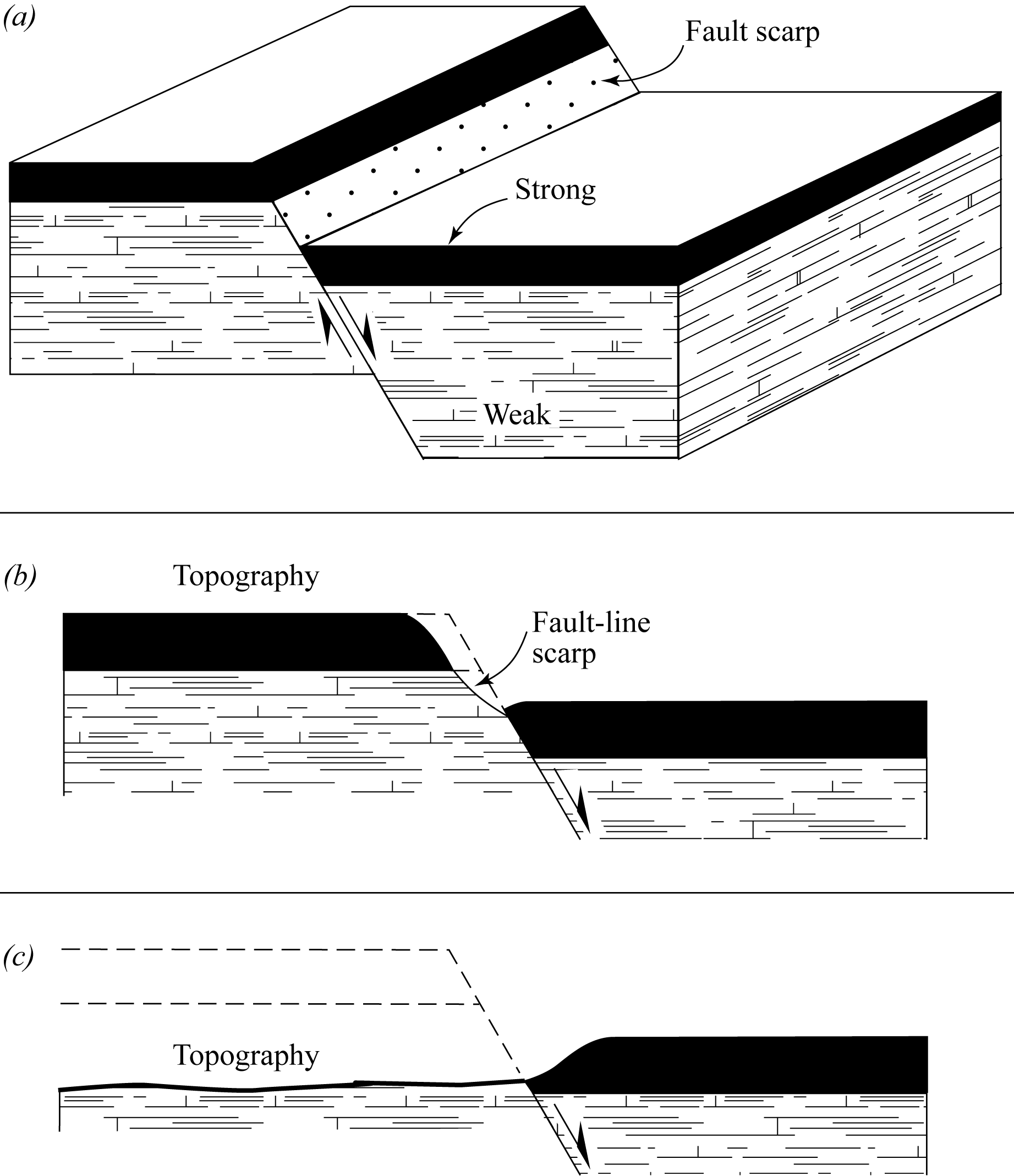
Figure 4.9. Topographic development by erosion

Topographically high areas commonly undergo more rapid erosion than do adjacent low areas. Thus, the highlands in Figure 4.9 (a) and (b) can become worn down, exposing the weak rock, which continues to erode faster than the strong rock on the adjacent downthrown side. The topography can become reversed with respect to the structure, in which case it is second-order topography. After considerable erosion and slope retreat, especially in second-order topography, the fault line may not necessarily be near the base of any escarpment. Sedimentation will further modify any of the above situations, Here, it is ignored for simplicity.

Figure 4.10 shows several first-order topographic features resulting from thrust faulting. Figure 4.10a shows a series of branching listric faults that elevate and rotate a layer of strong rock (stippled), thrusting it over a weaker rock. After erosion, the strong layer forms a series of ridges, and the weaker overlying rock sits in the valleys. In such cases, the thrust fault commonly lies along one side of the valley, and the other side leads onto the dipping face (dip-slope) of the strong rock.

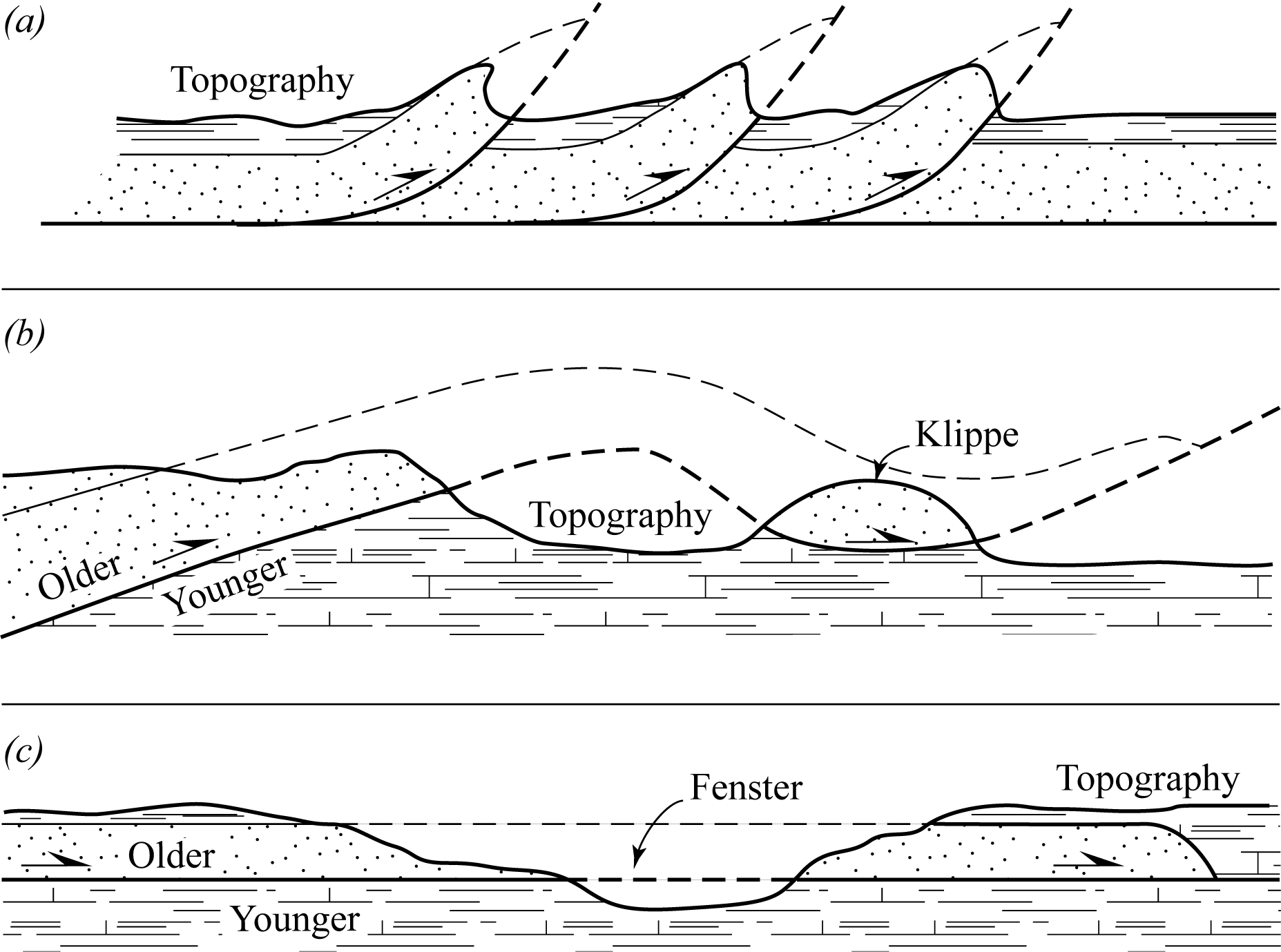
Figure 4.10. Variations of first-order topography

Figure 4.10b shows a slightly more complex situation in which the antiformal portion of a folded thrust fault has been cut away by erosion. This is most likely to happen if the footwall rock is weak. On the left, a typical thrust-fault type of fault-line scarp forms where older rock overlies younger rock. On the right is a hill or mountain formed as an erosional remnant of the nappe or thrust sheet (in this case in the synform). The isolated remnant is called a klippe. Figure 6.98 (Davis, Reynolds, & Kluth, p. 306) shows a klippe formed without folding.

Figure 4.10c shows how an erosional valley might cut through a laterally extensive thrust sheet, locally exposing the underlying younger rock in a relatively small area. Such a feature provides a window or fenster into the footwall rock, which we might otherwise never see.

The following figures illustrate thrust-fault-controlled topography in the southern Canadian Rocky Mountains.

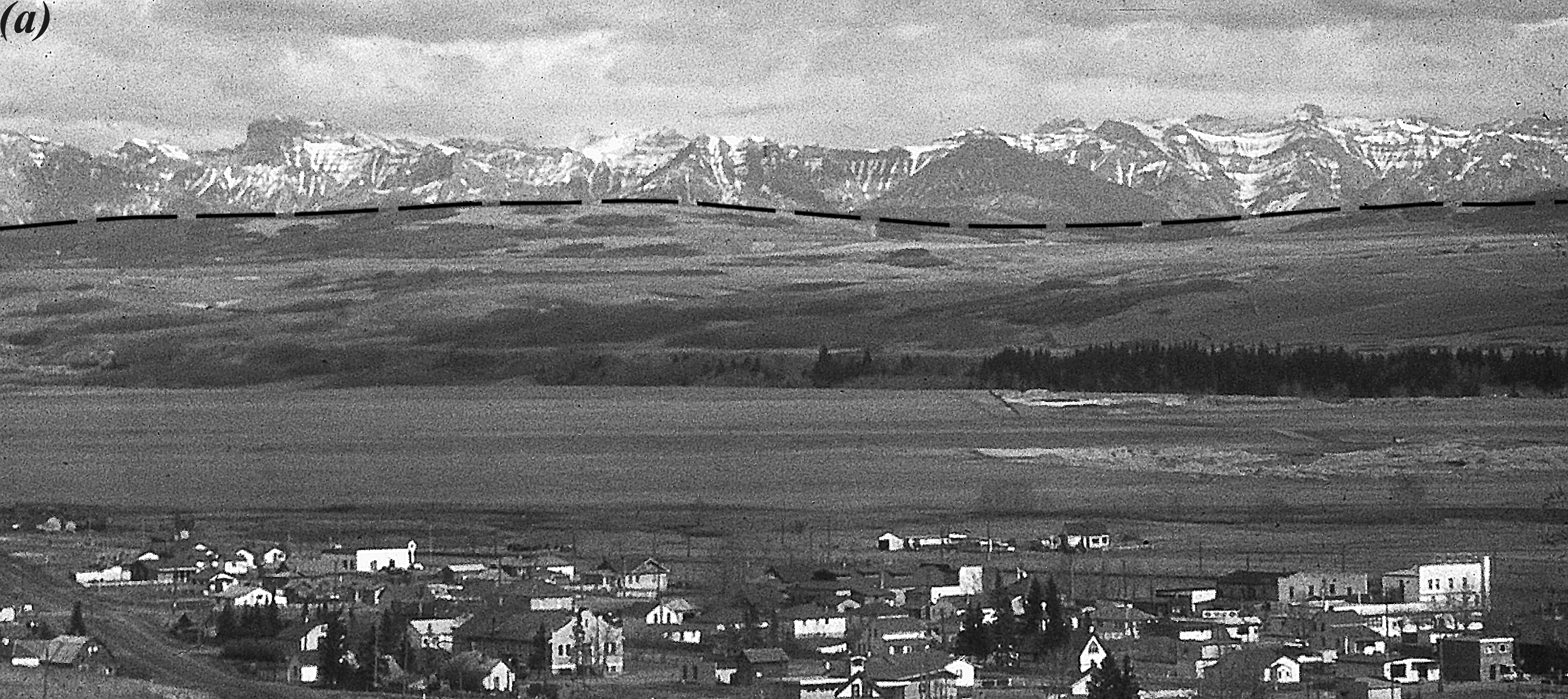
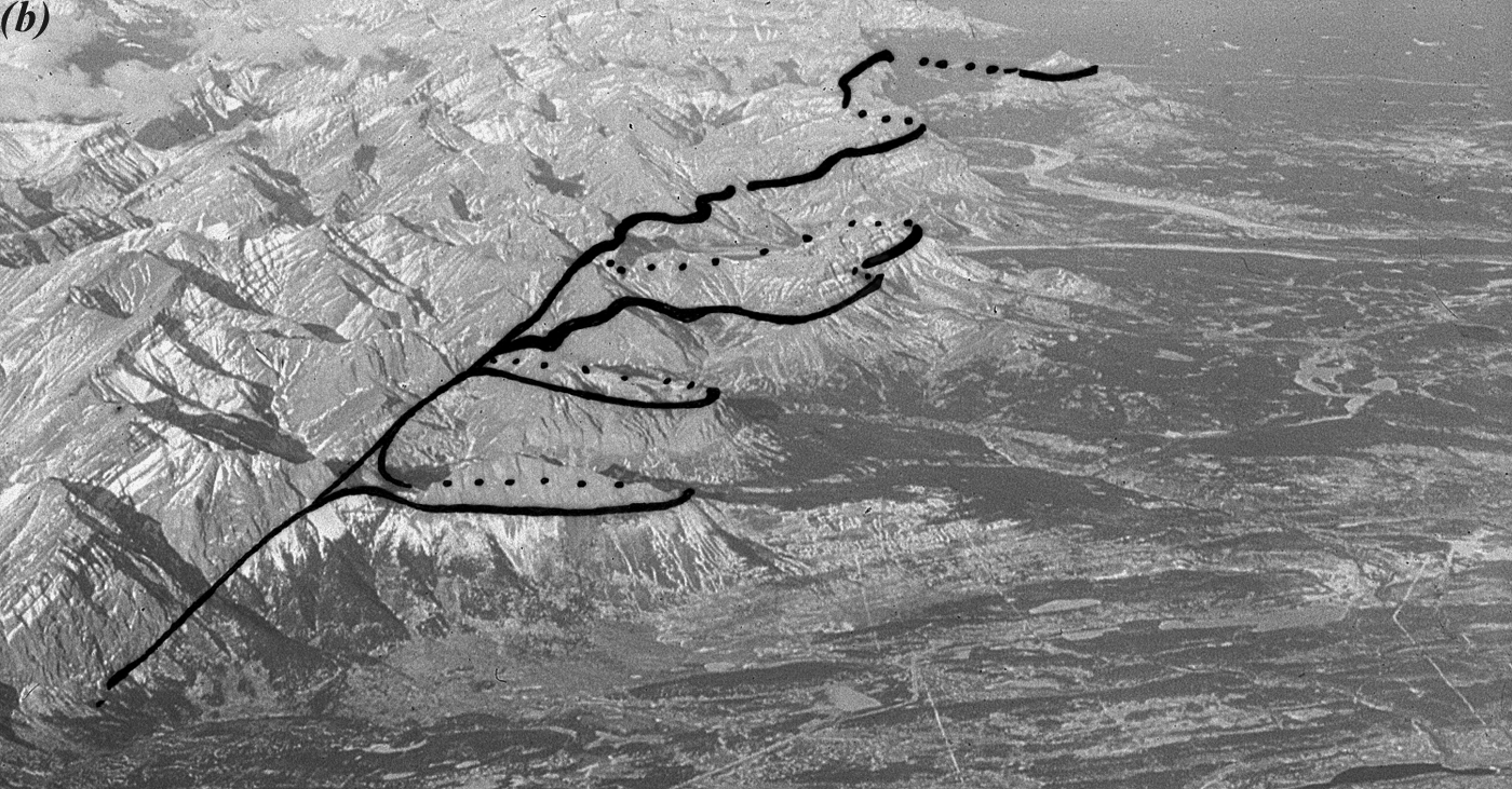
Figure 4.11. McConnell Thrust Fault

Figure 4.11a looks west into the Front Ranges of the Canadian Rocky Mountains (photograph taken from the Old Coach Road). Houses in the foreground are in the town of Cochrane, ~35 km west of Calgary, Alberta. The McConnell Thrust Fault (fault line shown by dashed line) dips to the west, and has brought Paleozoic limestone (mountains) over Cretaceous shales and sandstone (low foreground). The tallest mountain is just over 1 km high.

Figure 4.11b looks northwest along the front (east) edge of the Front Ranges (photograph taken from an aircraft while flying directly over the entrance of the Trans-Canada Highway into the mountains). The mountains shown here are just south of those in (a) and directly along the strike. Here, the McConnell Thrust (black continuous and dotted line) has undergone about 15 km slip. The fault and the rocks it cuts have been folded so that it dips to the west, making it nearly horizontal as it emerges from the mountains. Streams have cut valleys into the footwall shales, causing the irregular fault-line pattern. The fault line is shown as a continuous line where it is visible in the photograph, but as a dotted line where it is hidden by a mountain or projected from a klippe (e.g., top centre) to the main fault line. To the west, the McConnell fault is underground, but to the east, the hanging wall limestones have been eroded away, exposing the shales, which now form foothills. The mountains are caused by differential erosion of the limestone and shale, but the present positions of these rocks are controlled by the thrust fault.

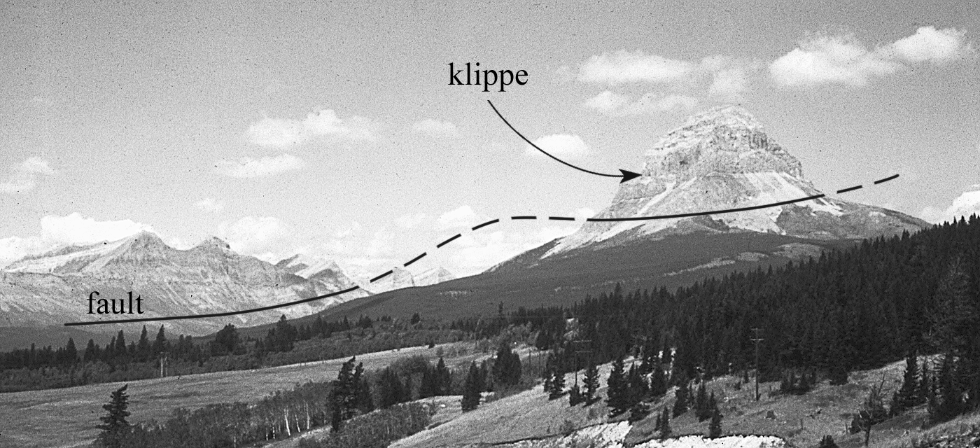
Figure 4.12. Crowsnest Klippe

The Crowsnest Klippe in Figure 4.12, the mountain on the right (0.5 km high), was formed by the incomplete erosional removal of Paleozoic limestone in the hanging wall of the Lewis Thrust Fault (black continuous and dashed line). Cretaceous shales, minor sandstones, minor tuffs, and minor but mineable coal seams occur in the footwall block. This structure is located in the Crowsnest Pass, near the Alberta-British Columbia border west of Lethbridge, AB. The fault is folded but dips generally to the west (left). It has undergone about 20 km of displacement at this site (overthrust to the east).

Study Questions

1. What is the difference between first-order topography and second-order topography?
2. How does second-order topography develop?
3. A depression eroded through a thrust sheet, exposing the footwall is called a ______________. An isolated remnant of a thrust sheet is called a ______________.

Lesson 7: Comparison of Brittle and Ductile Faulting

The features of faults discussed so far do not take into account whether faulting was brittle or ductile. From a human perspective, this difference is important, because brittle faulting (sometimes called seismic faulting) produces earthquakes, whereas ductile faulting (aseismic faulting) does not. Also, because rocks deform differently in brittle and ductile faults, the deformation fabrics of rocks within the two types of fault zones also differ.

7.1. Brittle versus Ductile Processes

Experimental studies of the ways in which rocks respond to stress under various temperatures, pressures, and water contents have shown that the time-stress relationships are quite different for brittle failure compared to ductile strain. Figure 4.13a demonstrates the plotting of generalized results: time is plotted on the x-axis, and stress difference (D = σ₁ − σ₃) on the y-axis. The diagram on the left side shows brittle failure, and the diagram on the right side shows ductile strain. In experiments, as in nature, a body of rock is subjected to stress (in experiments the stress results from hydraulic rams, and in nature from moving tectonic plates), and the response of the rock is monitored.

In the case of brittle failure, the rock first undergoes elastic strain as D (stress) is increased. The stress builds up until the rock reaches its elastic limit—the point at which it can no longer distort elastically. The rock then breaks, releasing the accumulated elastic strain. Except for the break, the rock regains its original shape (elastic recovery).

When the rock breaks, the applied stress difference drops rapidly, perhaps even to zero. If the rams continue to move, the elastic strain will build up again within the rock. However, the rock is now weaker, so its elastic limit is lower. It will break again, often along the original crack. Brittle strain, then, takes place in a series of breakages, separated by periods of time during which there is a slow accumulation of elastic strain. The accumulated elastic strain can be thought of as a form of stored energy; the more elastic strain that accumulates, the more energy is released by breakage, and the more violent the eventual breakage will be.

You can conduct a simple brittle-failure experiment yourself by using a small, thin piece of wood (such as a Popsicle-stick, twig, cheap ruler, pencil, or a bendable scrap of plywood). Slowly bend the stick without breaking it. Note that bending becomes progressively harder to continue as strain increases, and that the stress difference must be increased. Now release the bending force, and note that the stick regains its original shape. (You did not surpass the elastic limit of the stick.) Now bend the stick again, and continue until it reaches its elastic limit and breaks. Note that once the break occurs, the broken segments go back to being straight. Elastic rebound has occurred following brittle failure of the stick.

Ductile strain is very different (Fig. 4.13a, right). The initial response to stress is a small amount of elastic strain (not shown); the rock reaches its elastic limit very quickly. After the elastic limit has been reached, the ductile substance dissipates the stress applied to it by undergoing continuous, steady, permanent strain. You can model this in an experiment, by slowly stretching or squeezing a putty-like substance.

7.2. Seismic versus Aseismic Faulting

In your experiment with brittle failure, you will have noticed that breaking the stick generated sound. You likely also noted a physical jolt through your hands and arms. Both phenomena are due to the sudden release of the stored elastic energy (i.e., elastic rebound). Whenever brittle faulting occurs, the transmission of released elastic energy through the Earth manifests as an earthquake.

Figure 4.13b shows how this process works. Before faulting, the rocks in the future fault zone undergo elastic stretching (exaggerated here) as the rock masses on opposite sides begin to move past each other. When it reaches its elastic limit, the stretched rock breaks, a fault forms (or an old fault is reactivated), and the stretched rock in the fault zone undergoes elastic rebound. Although it is tempting to think of the breaking as near-instantaneous fault slippage, in reality, the rock masses had already moved. The fault slippage is really just the previously stretched rock regaining its original shape near the fault. The distorted segments become realigned with their undistorted extensions, which are now offset across the fault. The elastic rebound causes rapid compressions (“C” in Fig. 4.13b) and rarefactions (“R”: stretching strains) in the rock, much like a plucked guitar string. This jolt-like energy propagates away from the region of elastic rebound as an earthquake.

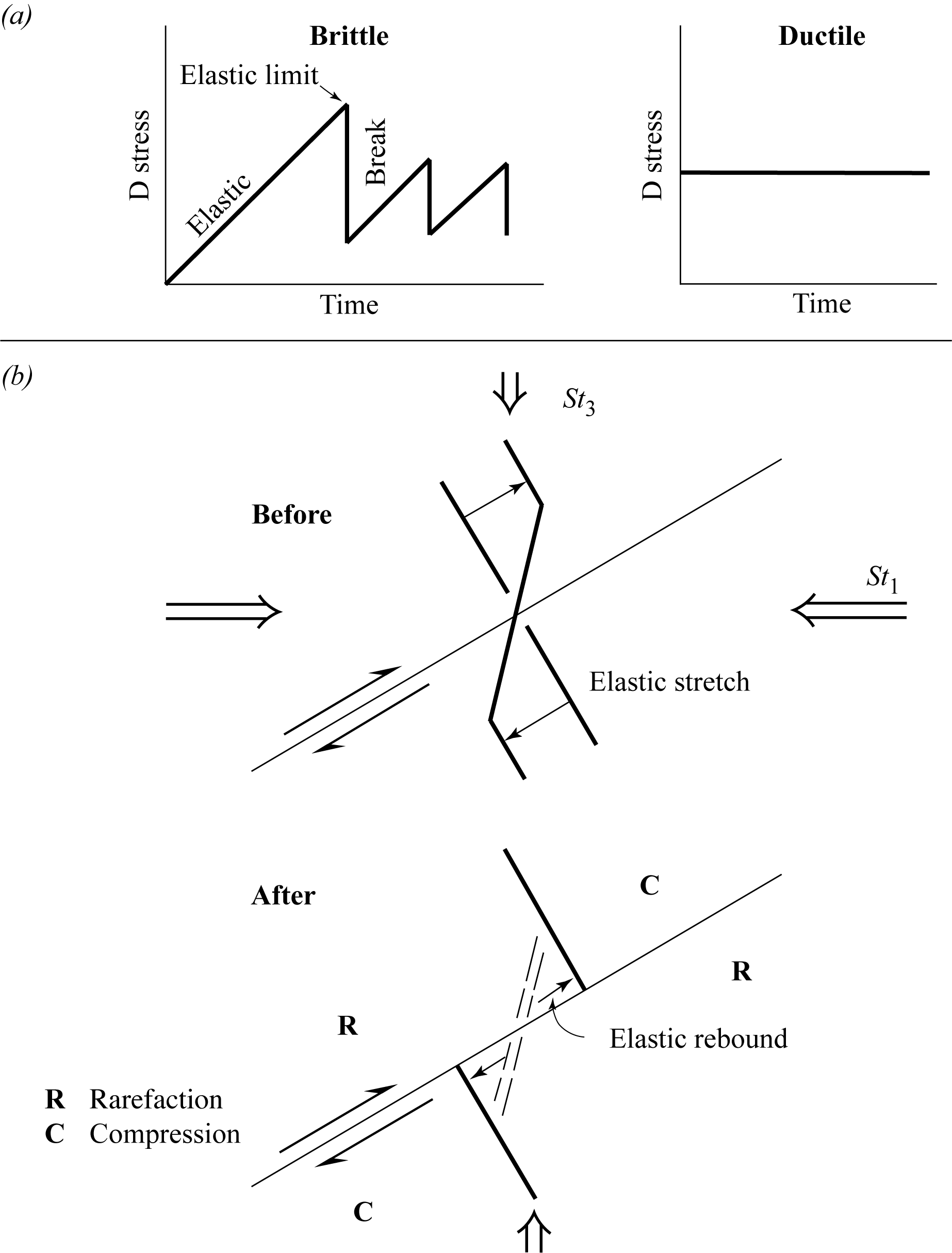
Figure 4.13. Brittle and ductile strain

To model a compressive, elastic-rebound-generated earthquake, place one hand on a table, and bend the fingers of that hand upward with the other hand (hopefully this is an elastic deformation!). Next, release the bent fingers down onto a table top (elastic rebound). This action will release sound (seismic) energy, and both you and the table will feel an earthquake-like jolt (however small). Slapping the table with one hand while feeling the table shake with the other can give you the general idea of the propagation of earthquake energy away from the point of brittle failure (the earthquake focus).

After undergoing elastic rebound, the rocks in the fault zone will again deform elastically, progressively storing strain until they reach their elastic limit once more, causing another rebound-earthquake event. All seismic faults behave this way: strain builds up over long periods of time, during which the fault is said to be stuck, then a brief, nearly instantaneous, rebound or slip event occurs. This is referred to as the stick-slip mechanism.

In contrast, ductile strain is steady and continuous. There is no stick-slip, no storage of elastic strain, and thus no elastic rebound. Therefore, movement along ductile faults does not produce earthquakes. The fault movement is termed aseismic.

Study Questions

1. What is the elastic limit of a material?
2. Why does brittle faulting cause earthquakes but ductile faulting does not?
3. What is the stick-slip mechanism?

Lesson 8: Introduction to Fault Rock

Small faults might be simple cracks in a rock across which differential movement has occurred. Large faults, on the other hand, always modify the rock in some way, producing fault rock. Fault rock occurs in fault zones that can vary in width from microscopic to several kilometres across. There is only a very general relationship between the amount of displacement and the width of the fault zone, so the width of a fault zone is a poor predictor of the amount of slip.

There are two broad categories of fault rocks:

• Brittle failure produces cataclastic rocks. The rocks in brittle fault zones are commonly highly fractured, with joints trending in a variety of directions, commonly forming an interwoven (or “anastomosing”) network approximately parallel to the fault.
• Ductile faulting produces mylonites.

8.1. Cataclastic Rocks

Cataclastic rocks form by the grinding and fragmentation of the faulted rock, a process called cataclasis. There are several varieties:

• Fault breccia consists of angular fragments of the wall rock, mostly greater than 1 mm in diameter, and some greater than a metre across. The spaces between large fragments are commonly filled with more-finely comminuted (mechanically broken) material (Davis, Reynolds, & Kluth, Fig. 6.26, p. 262).
• Fault micro-breccia forms from a more intense cataclasis, and contains no fragments larger than 1.0 mm across.
• Fault gouge is the result of even greater comminution. Rock is reduced to a granular material of flour-like consistency, with no particles larger than 0.1 mm across.

Fault breccia, micro-breccia, and fault gouge that form close to the Earth's surface (< 5 km depth) are initially highly porous and cohesionless, but can become cemented or sealed when groundwater percolates through pore spaces, facilitating crystal growth within the pore spaces. Mineral deposits such as copper and gold can form in this way.

Under slightly higher temperature and pressure conditions, cataclasis can produce a fine-grained material whose fragments are compacted and welded together virtually as they form. The result is a cohesive fault rock called cataclasite (not cataclastite). Cataclasites differ from fault breccia, microbreccia, and gouge primarily in that they do not require a secondary cement to be cohesive.

Cataclastic fault rocks are generally not foliated; that is, they are not layered. In some rare cataclasites, only a weak fragment alignment occurs.

8.2. Mylonite

Mylonite forms through extreme ductile deformation in rocks undergoing faulting under metamorphic conditions (i.e., temperatures higher than 300°C and pressures greater than those generated by approximately 5 km burial). Brittle crushing is not involved in the formation of mylonites.

Several features characterize mylonite, regardless of the lithology of the original rock (protolith) from which it forms:

• Mylonites are banded, (Fig. 4.14, Study Guide) with layers varying in mineral content, grain size, and, in some cases, grain shape.
• Many of the component mineral grains are highly elongate, producing foliation planes called S-surfaces (Fig. 4.15, Study Guide). Stretched-out quartz ribbons are a common feature in quartz-rich mylonites.
• A marked reduction in grain size occurs, with the final grains commonly being less than 1/10 their original diameter.

In some fault zones—especially under brittle-ductile transition conditions—frictional heat generated by rapid slippage causes thin seams of the fault rock to melt. The melt freezes quickly, forming a glassy material called pseudotachylite (Davis, Reynolds, & Kluth, Fig. 6.35B, p. 266).

For more images of fault-zone rocks, see Figure 11-24 (Marshak & Mitra, p. 228).

Reading Assignment

• Read Davis, Reynolds, & Kluth: “The Nature of Shear Zones” up to “Geometries” (pp. 530-533)
• Read Davis, Reynolds, & Kluth: “Brittle Fault Rocks” (pp. 260-267)
• Read Davis, Reynolds, & Kluth: “Foliations in Mylonitic Rocks” (pp. 499-501)

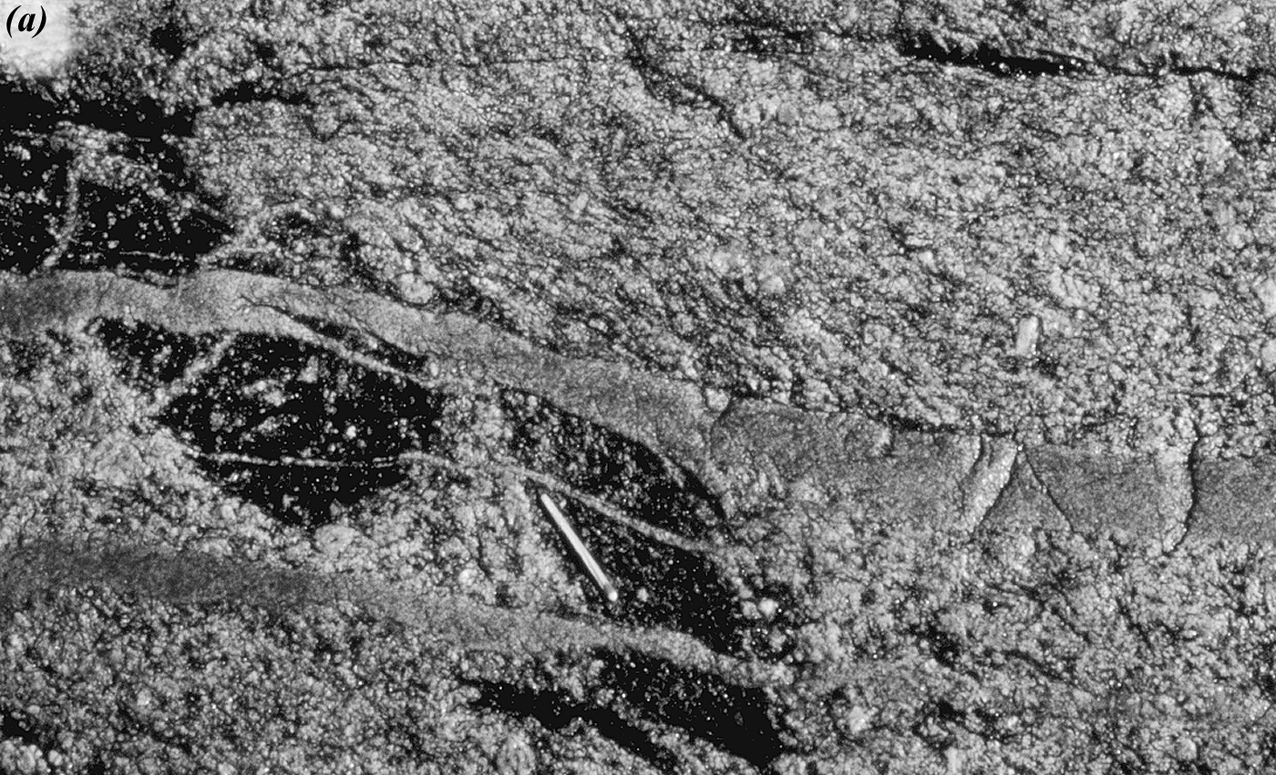
Figure 4.14. Banding in mylonites.

(a) Undeformed granite from the Proterozoic Wathaman Batholith in northern Saskatchewan, Canada. This is a typical outcrop of a large magmatic intrusion. The granite is undeformed except for small fractures. It contains two dark xenoliths, and is cut by veins of feldspar and quartz. Note the matchstick on one of the xenoliths, for scale. This type of rock is cut by several ductile faults, which strongly modify the fabric of the rock elsewhere.

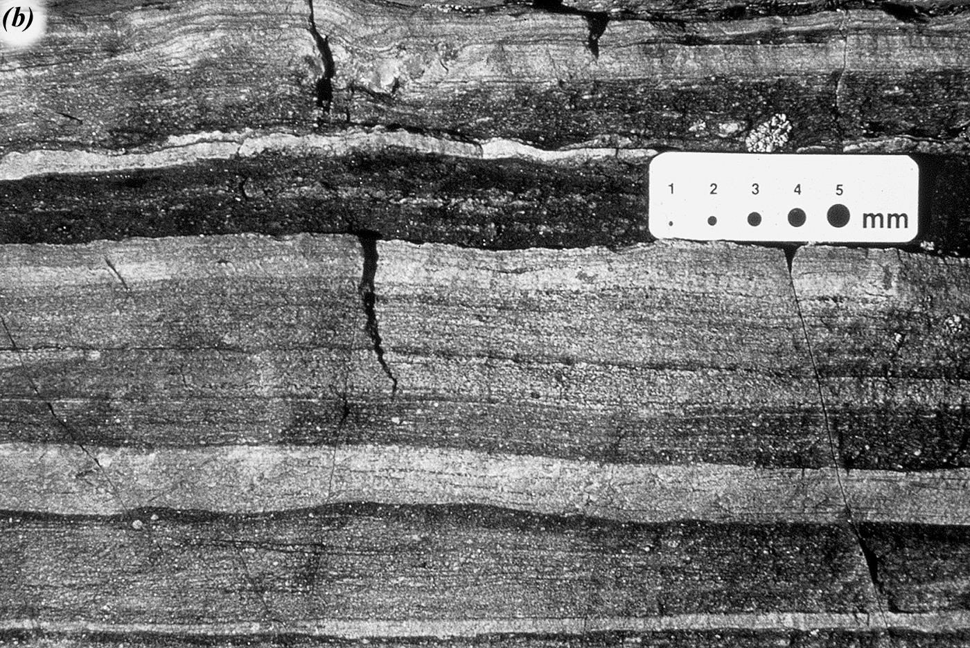
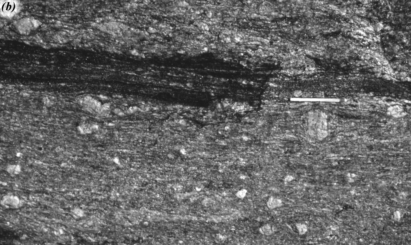
Figure 4.14. Banding in mylonites, cont.

(b) Deformed mylonite from Needle Falls Shear Zone, a major ductile fault that cuts the Wathaman Batholith. Fabric elements include colour layering, where darkest layers are stretched-out xenoliths, the lightest two layers are stretched-out veins, and the medium-colour rock is the host granite. The streaky appearance of all of the rock types is caused by stretched-out feldspar and quartz grains that have been rotated parallel to the layers.

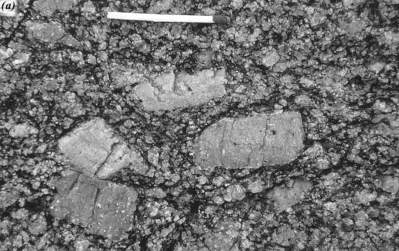
Figure 4.15. Development of S-C fabric in Wathaman Batholith.

(a) Large phenocrysts in undeformed granite. Note matchstick for scale. Rock similar to this is affected locally by ductile shear zones.

(b) Moderately developed S-planes produced in a ductile shear zone cutting part of the Wathaman Batholith. Groundmass feldspar and quartz grains have been stretched, yielding a streaky-looking outcrop. S-planes dip nearly vertically and strike E-W. The orientation can be approximated by holding your hand straight along this streaky pattern and perpendicular to the photograph. The largest phenocrysts are affected little by deformation at this locality. This rock is not deformed enough to be called a mylonite, but could be referred to as a protomylonite. Note matchstick for scale.

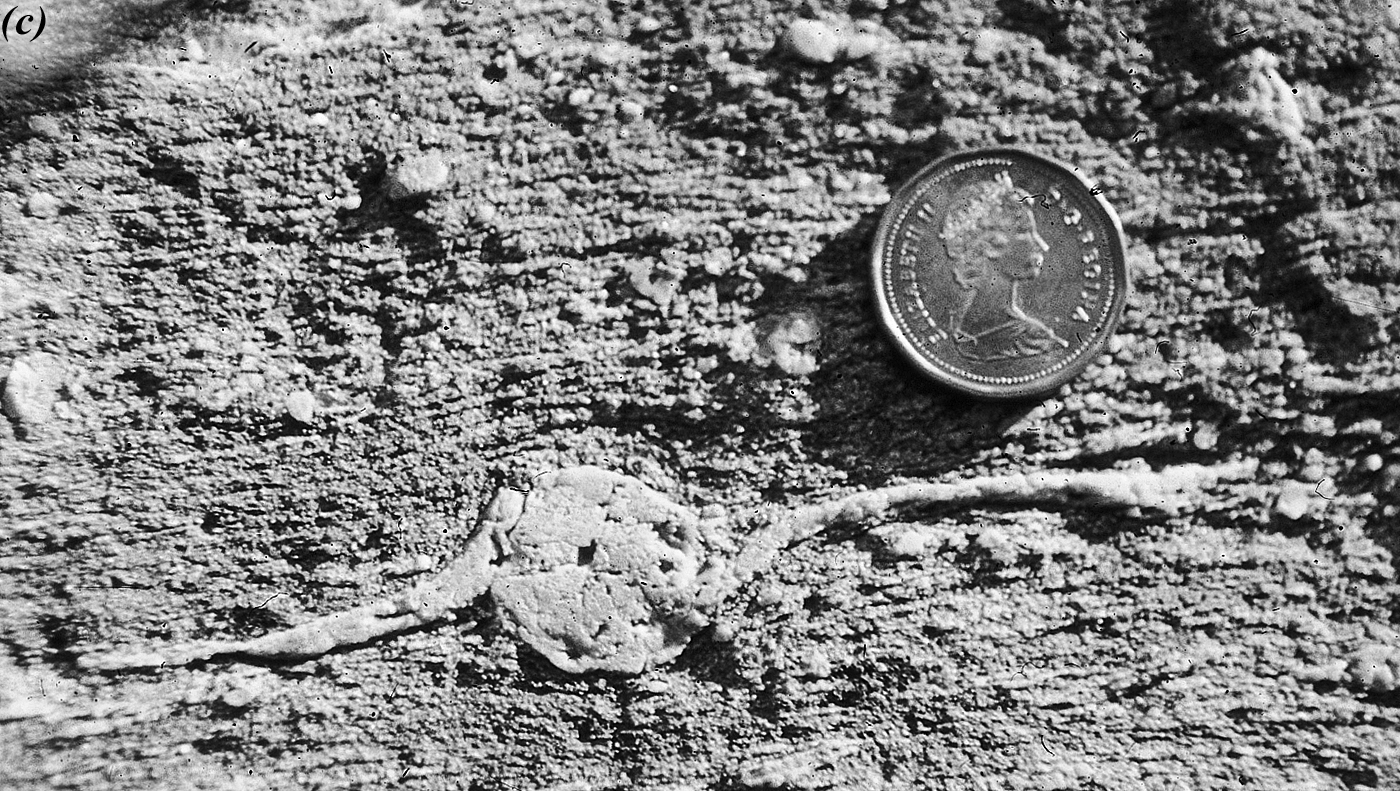
(c) Deformed,well-developed protomylonite from the Needle Falls Shear Zone. S-C fabric (S and C parallel here) and rotated phenocryst both show dextral shear or clockwise rotation. Note penny for scale.

Figure 4.15. Development of S-C fabric in Wathaman Batholith, cont.

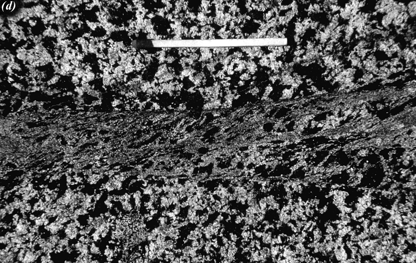
(d) Deformed: Small ductile fault cutting diorite from a pluton in northern Saskatchewan. The fault zone is vertical, and perpendicular to the photograph. The S-fabric is oblique to the sides of the shear zone, and there are internal C-bands parallel to the shear zone.

Figure 4.15. Development of S-C fabric in Wathaman Batholith, cont.

8.3. Slip Indicators in Fault Rock

Brittle Faults

Some brittle fault surfaces become highly polished by the abrasive slip of one rock mass past the other, producing a polished surface called a slickenside. It is common for groundwater precipitation to cause veining along the fault surface (in which case the side of the vein will be slickensided) or to cause staining of the rock (in which case the stain—commonly iron hydroxide—may be polished). Slickensides are commonly striated on the mm to cm scale (see Fig. 4.16, Study Guide) as a result of

• scratches on the surface, running parallel to slip (Fig. 6.11, Davis, Reynolds, & Kluth, p. 254), or
• needle-like mineral growth (usually quartz or calcite), parallel to slip (Fig. 6.14, Davis, Reynolds, & Kluth, p. 256).

These striations are commonly called slickenlineations, although they can occur without the polish of the slickenside. The fault surface may also be grooved parallel to the striations (Fig. 4.16b; Fig. 6.11, Davis, Reynolds, & Kluth, p. 254). Striations and grooves are useful for determining the direction of fault slip, but not the sense of slip. That is, slip was parallel to the striations (direction of slip), but one cannot tell how one side of the fault moved with respect to the other (sense of slip).

Slickenlineations commonly occur with small (mm- to cm-scale) steps in the fault surface that may be either small chattermark-like features (Fig. 4.16a), or bundles of vein crystals (Fig. 4.16c). These steps result in the formation of small gaps (seen in the cross-section in Fig. 4.16d) that may fill with breccia, gouge, or vein material. The steps are useful for determining the sense of slip because their faces always point opposite the direction of motion. Applying this indicator to Figure 4.16 (a and c), we can conclude that the rock mass has moved away from the viewer in both cases.

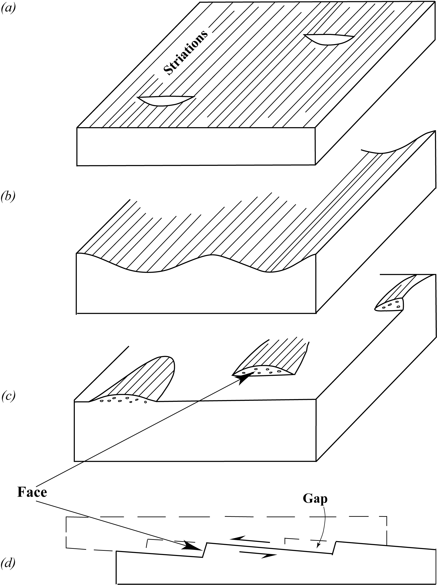
Figure 4.16. Brittle fault slip indicators

Reading Assignment

• Read Davis, Reynolds, & Kluth: “Slickensides and Slickenlines” up to “Fault Zones” (pp. 254-259)

You can find more images of slickenlineations in Figures 11-26 and 11-27 (Marshak & Mitra, pp. 230-231).

Ductile Faults

Ductile faults and brittle-ductile faults develop a number of features that are useful as kinematic indicators. Here, we will study only those features that result from ductile distortion of grains.

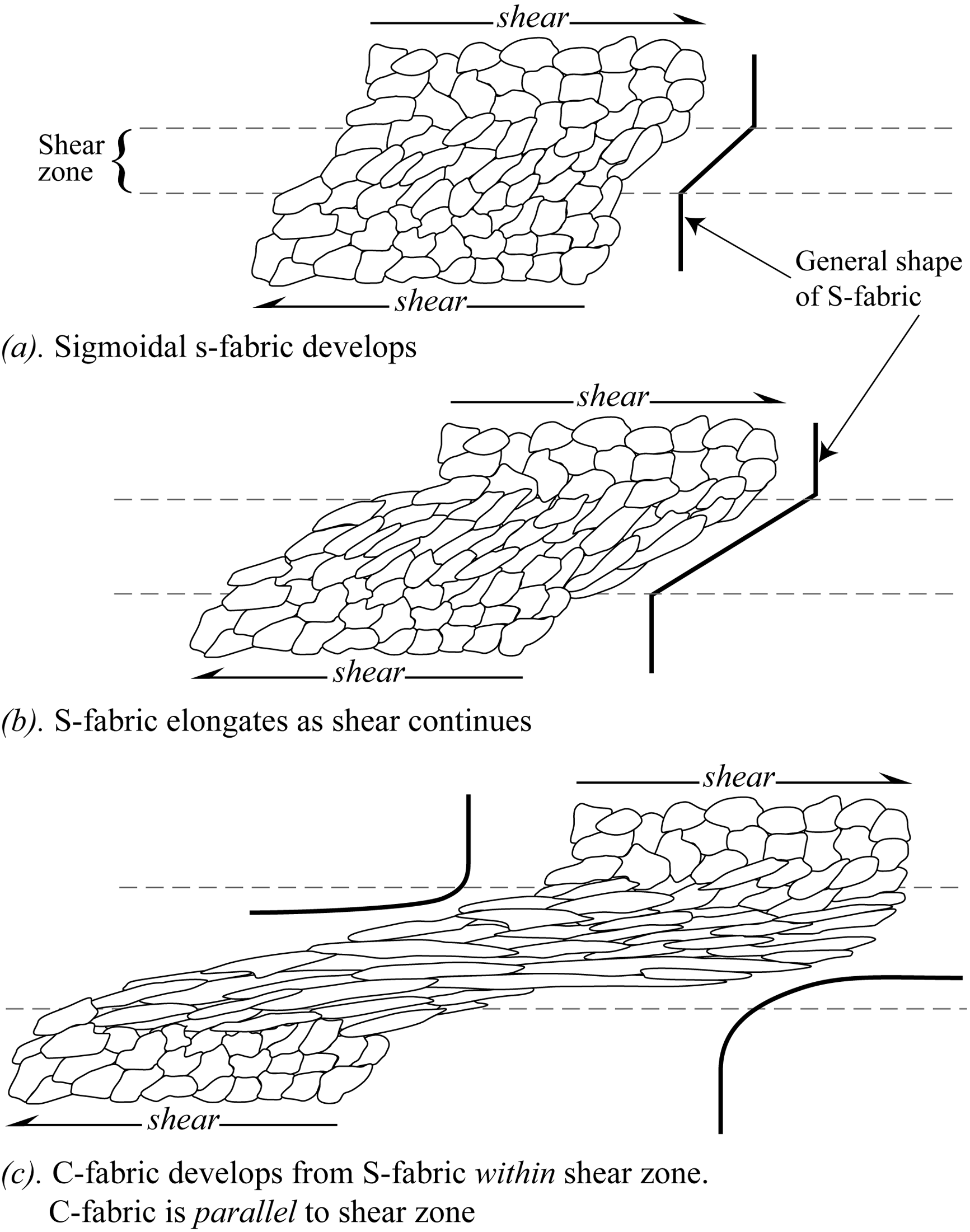
Figure 4.17. Grains stretching into S-fabrics and C-fabrics

Ductile stretching causes component grains to become elongate, and eventually to be oriented along the slip direction. Figure 4.17 shows how grains first become stretched obliquely to the fault, then progressively rotated into parallelism with the shear. The plane in which the grains originally become stretched is referred to as the S-fabric (stippled surfaces in Fig. 4.18 (a, d). The S-fabric curves towards the direction of shearing, called the C-fabric (Fig. 4.18). The sense of rotation indicates the sense of shear, or slip.

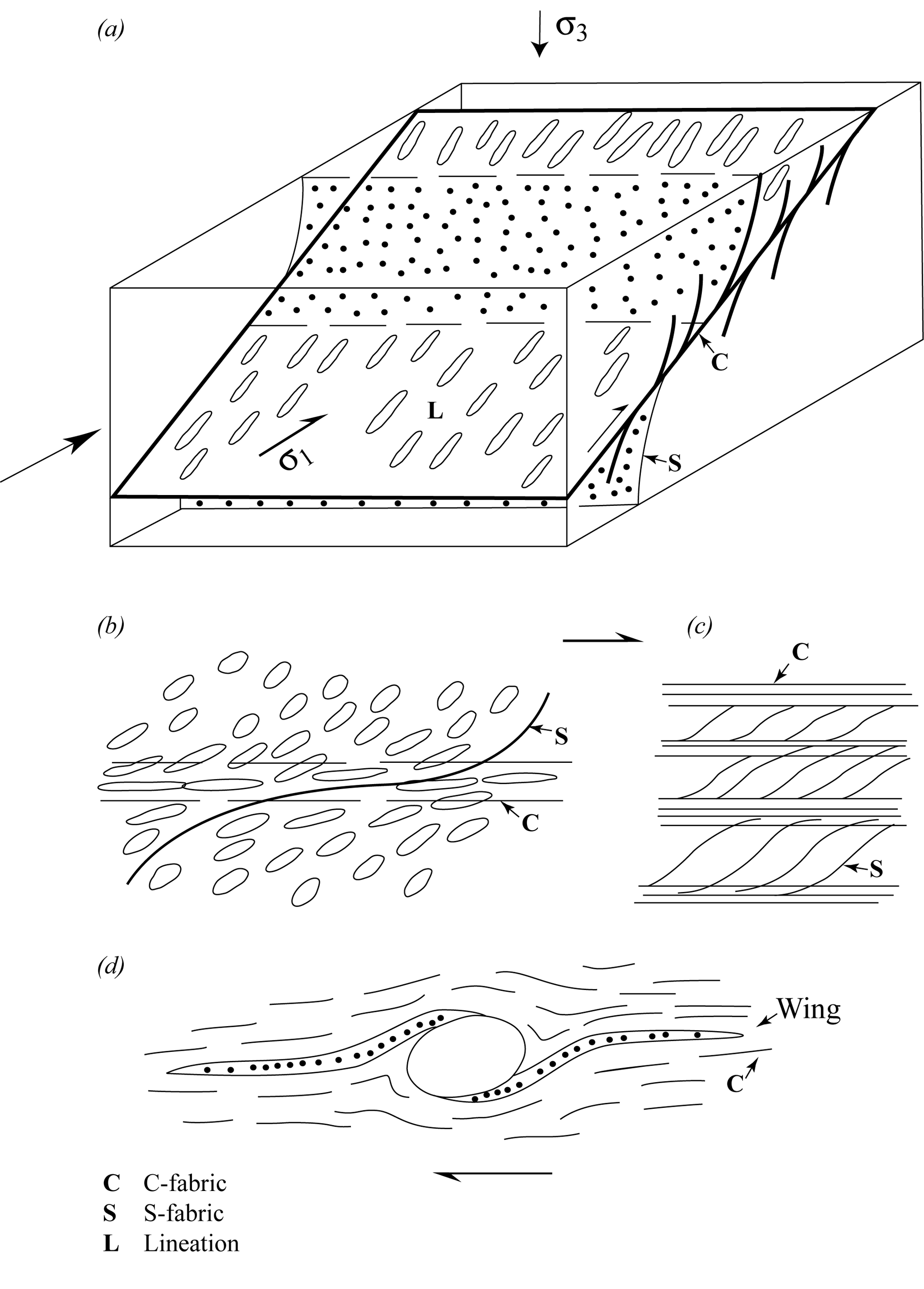
Figure 4.18. Fabrics resulting from ductile deformation

Stretched grains take on the shape of flattened cigars (with oval cross-sections), and their lengths form a lineation (L) nearly parallel to the direction of slip (Fig. 4.18a). Lineation is parallel to the S₁-axis of the strain ellipsoid, and the S-planes are parallel to the S₁S₂ plane of strain.

Where S becomes parallel to C, the stretched grains are highly elongate, and L is perfectly parallel to the direction of slip. Any one outcrop may display either S- or C-fabric. If they occur together, the combined structure is called an S-C fabric (Fig. 4.18cand d). C, S, and L fabrics are very important for the analysis of ductile shear zones, because together, they permit the direction and sense of slip to be determined.

Large grains, such as phenocrysts in granite plutons, may develop wings pulled off the host grain, which help to form the lineation and the C-fabric. The phenocrysts may become rolled in the sense of shear (Figs. 4.15c, 4.18d), or deflected into C.

For more examples of what these ductile kinematic indicators look like, turn to Figures 11-30 and 11-31 (Marshak & Mitra, pp. 234-235).

Reading Assignment

• Read Davis, Reynolds, & Kluth: “Foliation Patterns,” up to “Mica Fish” (pp. 559-563)
• Read Davis, Reynolds, & Kluth: “Inclusions” up to “Pressure Shadows” (pp. 564-565)
• Read Davis, Reynolds, & Kluth: “The Origin of S-C Fabrics” (pp. 583-585)

Study Questions

1. What is the difference between cataclastic rocks such as fault breccia and fault gouge, and cataclasite?
2. What is the difference between direction of slip and sense of slip?
3. How can you determine the direction and sense of slip in a brittle fault zone?
4. How can you determine the direction and sense of slip in a ductile fault zone?

Assignment 4

You should now complete the theory portion of Assignment 4, which you can find in the assignment drop box. You will submit this assignment to your tutor for grading after you have also completed the lab portion.

Answers to Study Questions

Lesson 1

1. Faults, joints, and fractures are all cracks in rock. A fault, however, is a crack across which there is differential movement. In other words, the rocks on either side of a fault move relative to each other.
2. Separation refers to the apparent movement along a fault that can be seen in map view or in outcrop, whereas slip refers to the actual movement. The distinction is important because separation can give an erroneous impression of what has happened along the fault. For example, if a normal fault or a thrust fault occurs in dipping strata, a map view of the eroded surface will show a horizontal offset between beds (giving the impression of a strike-slip fault), even if no horizontal motion has occurred. Separation does provide useful data, however. In the lab component of this course, you will learn techniques for using these data to determine the slip.

Lesson 2

1. The important stress for causing a normal fault comes from gravity acting on the rock mass, rather than tension at the Earth's surface. Gravity acts in a downward direction, so the maximum principle stress is vertical. It follows then, that for a thrust fault to form, the compressive stress acting on the rocks must be greater than the stress due to gravity.
2. True. The material properties of rock (i.e., the 30° angle of internal friction) mean that a high-angle fault cannot form at the Earth's surface under a compressive stress regime. Nonetheless, a reverse fault can occur at the Earth's surface if compression causes a normal fault to be reactivated.

Lesson 3

1. Thrust faults cause thickening and shortening of Earth's crust.
2. The basement rocks are decoupled from the rocks above by a decollement in a layer of weak rock. As a result, compression may fold and fault the rocks above the decollement, but this force is not transmitted to the basement rocks below.
3. Steps and ramps are present when a thrust fault cuts through rocks of different strengths. When it cuts through a stronger layer, the dip of the thrust fault is steeper, forming a step. When it cuts through a weaker layer, the dip is not as steep, and it forms a ramp.
4. Fluids contained within rocks can be under very high pressures, which can counteract the force of gravity on the rocks above. The high fluid pressure has the same effect as decreasing the mass of the rocks. In fact, the pressure can be so high that it nearly cancels out the effect of gravity. In this case, a relatively small amount of force is required to overcome friction along the fault and to move the thrust sheets.

Lesson 4

1. Normal faults cause thinning and extension of the Earth's crust.
2. Many geologists thought that the mechanical properties of rocks precluded the existence of low-angle normal faults. Therefore, geologists tended to label all low-angle faults as thrust faults.
3. Some low-angle normal faults started out as higher-angle normal faults, but the fault blocks became tilted and rotated as the basin in which they formed grew wider.

Lesson 5

1. True.
2. At the bends and jogs of strike-slip faults, one of two things can happen: parts of the fault can collide with each other, causing topographic highs, or parts of the fold can move away from each other, opening up a hole in the Earth's crust (e.g., Fig. 6.146B, Davis, Reynolds, & Kluth, p. 339). The hole, called a pull-apart basin, can accumulate large quantities of sediment. Pull-apart basins, such as Death Valley in California, have some of the lowest elevations on the surface of the Earth. (Note: Death Valley is also classified as a half-graben, because normal faulting occurs within the hole created by the strike-slip fault.)

Lesson 6

1. First-order topography is shaped like the structure that created it. After modification by geological processes, topography may still exist because of the structure, but the topography may no longer resemble the original structure. This is referred to as second-order topography.
2. Second-order topography can form when a structure consists of rock layers of differing strength. Erosion will proceed more rapidly in the weaker rocks than in the stronger rocks. The resulting topography will be controlled not by the original shape of the structure, but by the relative strength of the rocks making up the structure.
3. A depression eroded through a thrust sheet, exposing the footwall is called a fenster. An isolated remnant of a thrust sheet is called a klippe.

Lesson 7

1. The elastic limit of a material is the level of stress after which deformation of the material is permanent. If stress is removed before the elastic limit is reached, then the material will go back to its original shape.
2. In a ductile material, once the elastic limit is reached, the material deforms in a uniform way, slowly releasing the elastic energy that was stored. In contrast, a brittle material breaks when it reaches its elastic limit. The important difference is that the elastic limit of the brittle material is exceeded in a limited area, where the break forms. Away from the break, the elastic limit of the brittle material has not been reached, so the bulk of the brittle material will spring back to its original shape once the stress is relieved by faulting. Therefore, it is the release of elastic energy as the rock snaps back to its original shape that creates an earthquake, not the fracturing of the rock.
3. The stick-slip mechanism is the repeated build-up and release of elastic energy in rock by brittle deformation.

Lesson 8

1. Fault breccia and fault gouge are formed in brittle fault zones at depths of less than 5 km below the Earth's surface. These fault rocks are initially very porous, and the particles do not stick together. (Groundwater can make them sticky or cement them together later.) In contrast, cataclasite is formed in brittle fault zones at depths greater than 5 km, and because of the higher temperatures and pressures, the particles are compacted and stick together immediately.
2. The direction of slip refers to the direction in which shear stress is oriented along a fault, whereas the sense of slip refers to how rocks on one side of the fault have moved relative to rocks on the other side.
3. In a brittle fault zone, slickenlineations give the direction of slip. The flat faces of chattermarks look opposite the direction of slip, so they can be used to determine sense of slip.
4. In a ductile fault zone, the direction and sense of slip can be determined from the orientation of deformed crystals in fault rocks. Over time, elongated crystals slowly rotate to be parallel to the direction of slip. The initial lengthening of crystals makes the S-fabric. The S-fabric is oriented diagonally across the fault zone; this gives the sense of slip. Inclusions within the rock can also be useful indicators of the sense of slip, because they rotate in the shear direction. If “wings” are pulled off of the inclusion, these provide a record of the direction of rotation.