Geology 319 Structural Geology: The Architecture of Earth’s Continental Crust

Lab Unit 5

Displacement on Faults

Overview

In this unit you will learn how to determine the amount and direction of movement, or slip, that a fault has undergone. Displacement on a fault may be linear, or it may involve rotation. In this unit we will restrict our focus to cases in which the movement along the fault is linear and the topography is flat.

In Lesson 1, you will learn the necessary terminology for working on faults. In Lesson 2, you will learn how to calculate the net slip on a fault given two bodies that intersect the fault. In Lesson 3 you will learn how to calculate net slip given one intersecting body plus information about slip lineations. Lesson 4 offers a practice exercise with a twist, to get you thinking about how to set up net slip problems.

Objectives

After completing this lab unit, you should be able to

1. determine the slip undergone by both vertical and dipping faults given
   1. two displaced planar bodies, or
   2. one displaced planar body and the direction of slip.
2. describe the relative motion, or sense, of a fault.
3. explain why a horizontal offset may be visible on a geological map even when a fault has not undergone a horizontal component of slip.

Materials

• Basic Methods of Structural Geology by Marshak & Mitra
• stereonet
• several sheets of 8½″ × 11″ plain, white paper
• several sheets of 8½″ × 11″ tracing paper
• protractor
• ruler
• pencil and eraser
• calculator

Lesson 1: Motivation and Terminology

What do we gain by calculating how much a fault has slipped? Why does it matter? There are several reasons:

1. Most faults form during orogeny. Their slippage was part of the orogenic process, so understanding how much they moved helps us understand how continental crust developed.
2. Plate tectonics operates in large part by slippage on faults. To understand plate tectonics fully requires that we understand fault displacement.
3. Plate tectonics has caused the sea floor to be broken by millions of faults. To understand the physical structure and evolution of ocean basins, we must understand fault displacement.
4. Many gas and oil fields are controlled or modified by faults.
5. Many ore bodies are cut and offset by faults. Sometimes it is necessary to determine how much a fault has slipped to locate other parts of an ore body.

Active brittle faults cause earthquakes when they slip. Knowing how much the fault has slipped in the past and how fast the opposite sides are moving now is useful information for predicting earthquakes.

There are a number of terms that describe how movement has taken place along a fault and how much movement has occurred. It is important that you understand these terms clearly.

Reading Assignment

• Reread Davis, Reynolds, & Kluth: “Displacement Vectors” and “Translation (Slip) on Faults” (pp. 47-51)
• Read Marshak & Mitra: “4-6. Descriptive-Geometry Analysis of Fault Offset” up to Problem 4-16 (p. 81). Pay special attention to Figures 4-19 and 4-20 (p. 82).

Your objective for these readings is to learn the following:

• What is the difference between net slip and separation?
• Seeing strike separation in map view does not guarantee that the fault in question is a strike-slip fault. Why? (See Fig. 4-20, Marshak & Mitra, p. 82)
• What is the difference between direction of transport and sense of transport? In your notes, include an example of each.
• What is relative displacement, and why is it necessary to describe fault movement by relative displacement?

Overview of the Process

In this lab you will learn how to use descriptive geometry and stereonet analysis to calculate the magnitude and direction of slip along a fault. In general terms, the approach is as follows: Imagine that you can pull the fault apart and walk along it. You can examine either side of the fault plane as though the fault blocks made up opposite walls of a hallway. If the fault happened to intersect a mine tunnel, for example, then you could measure the magnitude and direction of slip by measuring how far and in what direction one part of the tunnel has moved from the other.

Of course, the point of reference you use does not have to be a tunnel—it could also be the intersection of geological structures. When viewed in the plane of the fault (i.e., on the walls of the hallway), these intersections are points. We will learn how to use two different sets of intersecting geological structures:

• In the displaced two-body situation, we will use two intersecting planes, such as two beds, or a bed and a dike.
• Alternatively, we can use the intersection between a line representing the orientation of slip linears (also, slip lineations, or slickenside lineations) and a plane.

You will use your descriptive geometry and stereonet skills to determine what the intersections would look like on the walls of your hallway (a two-dimensional representation, like a painting hanging on the wall), where you can perform measurements on them.

Lesson 2: The Displaced Two-Body Situation

Case I: Vertical Fault, Flat Topography

A thin vertical dike striking 090° cuts the contact between thick sandstone and shale formations, which strike 045° and dip 40°SE. These are cut and displaced by a vertical fault striking 000°, as shown in Figure 5.1a (labs). Determine the fault displacement by measuring

1. the magnitude of net slip
2. the rake (or pitch) of the slip line
3. the relative movement

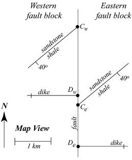
Geological map showing the fault, the contact between sandstone and shale, and the dike.

Figure 5.1. Case I, displaced two-body situation with vertical fault and flat topography

A three-dimensional view of this scenario is shown in Figure 5.2a (labs). This view shows you the block on the western side of the fault. The front of the drawing shows you the view that you would have on the western wall of the hypothetical hallway. Notice that in the plane of the fault, the two planes representing the dike and the contact appear as lines. These lines are called traces. TC_w refers to the trace of the contact on the western side of the fault, while TD_w refers to the trace of the dike. The point W is at the intersection of the traces.

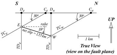
Figure 5.2b shows the traces of the contact and the dike from both the eastern and western sides of the fault. The view in Figure 5.2b is a profile of the fault surface, which is called the true view. Notice that the traces of the contact and dike on the eastern side of the fault, TC_e and TD_e, respectively, intersect at the point E. The offset between W and E is the net slip of the fault.

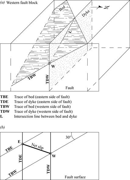
a) Three-dimensional diagram with traces of the western segments of the contact and dike.

b) True view showing traces of eastern and western segments.

Figure 5.2. Visualizing the displaced two-body situation

How to Draw the True View

1. Draw a line to represent the top of the true view. This line is sometimes called the folding line, because if you were to fold your page downward at 90° along the folding line, the vertical part of your page would be in the same orientation as the fault. Using tick marks, transfer the positions of the planes along the fault (points C_e, C_w, D_e, D_w) from the map view (Fig. 5.1) to your line (Fig. 5.3a).
2. Using your stereonet, find the rake of the contact and the dike in the plane of the fault. Notice that the fault is perpendicular to the strike of the dike, so the rake of the dike in the plane of the fault is the same as the dip of the dike: 90°. The fault is not perpendicular to the strike of the contact, so the trace of the contact will not show the true dip (40°SE). Instead it will show the apparent dip (30°S). Notice also that the intersection between the dike and the contact on the stereonet is the line, L, shown in Figure 5.2a.
3. Draw the traces onto the true view using the rakes you measured on the stereonet. (Fig. 5.3c). Label the traces clearly so you know which traces are the contact and which are the dike, which traces are on the west side of the fault, and which are on the east. Draw a point where the two western traces intersect and another where the two eastern traces intersect. Connect the points with a line. The length of the line is the magnitude of net slip. In this example, the net slip is 1.55 km.
4. Measure the rake of the slip line by measuring the angle of the segment EW down from the horizontal. The rake of the slip line is 18°N. The direction of the slip can also be expressed in terms of plunge and trend. Returning to the stereonet, plot the rake of the slip line, and then measure the plunge and trend (Fig. 5.3b).
5. The relative movement describes which way the fault blocks have moved compared to one another. In reality, it is difficult to say in absolute terms what the movement of each block was. One block may have stayed fixed, or the blocks may have moved in opposite directions. The blocks may even have moved in the same direction, with one block moving more than the other.
6. Relative movement is determined by inspecting the true view drawing of the fault, (Fig. 5.3c) and describing how one of the reference points has moved compared to the other. If we arbitrarily keep the western block fixed, then the relative movement is that the eastern block moved up and to the south with respect to the western block. Equally valid, we could say that the western block moved down and to the north with respect to the eastern block.

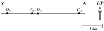
a) Step 1: Draw the top of the profile and transfer the plane positions from the map

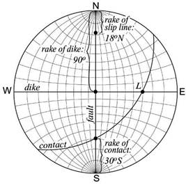
b) Step 2: Use your stereonet to find the rake of the traces on the fault plane.

c) Step 3: Draw the traces and mark the points where the eastern traces intersect (E), and where the western traces intersect (W).

Figure 5.3. How to draw the true view for Case I

Why can't I just measure the offset of the contact or dike from the map?

Look back at the geological map in Figure 5.1a. Notice that the strike separation of the contact and the dike are not equal. The dike appears to have been offset less than the contact. This is because the fault underwent a component of dip slip, which brought regions originally at different elevations to the same level. The distance between the contact and the dike increases with depth because the contact is dipping away from the dike. Therefore, the dip-slip component brought a region to the surface where the contact and the dike were further apart.

The strike separation will only be equal in two cases:

• when the traces of the two planes on the fault are parallel. Parallel lines will never intersect, so they cannot be used to solve for net slip.
• when the fault has undergone slippage in the strike direction only. In this case, the correct approach is to measure the offset from the map.

Case II: Dipping Fault, Flat Topography

If the fault is dipping, it is necessary to account for the dip when calculating the traces. Fortunately, by using the stereonet to calculate the rake of the two planes on the fault (step 2, above), the dip of the fault plane is automatically factored in.

You will draw the true view in the same way that you did before. Remember that the true view is always drawn as though the fault plane has been rotated upward to the horizontal. Therefore, there is nothing to adjust here, either.

Practice Exercise

Problem 6-15 (Marshak & Mitra, pp. 120-122) is a worked example of Case II. Try to do the problem yourself before reading the description of the solution. Note that the point X is labelled in a confusing way in Figure 6-17c (p. 121). X refers to the point on the fault that marks the slip line (discussed in step 6 of Problem 6-15), not a point on the primitive circle. Also note that it is entirely coincidental that the trend of the slip line is the same as the strike of the dike (Fig. 6-17c).

Lesson 3: Fault Solutions Using Slip Lineations

If slip lineations (or slip linears) are present, then net slip can be determined with only one displaced planar structure. This is because the slip linear has the same orientation as the net slip. Like the displaced two-body situation, the method is the same for both vertical and inclined faults.

a) Geological map showing the quartz vein and the fault

Figure 5.4. Case I, displaced two-body situation with vertical fault and flat topography

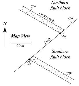
Consider the following example: A fault with strike and dip of 050°/60°NW cuts a gold-bearing quartz vein with attitude 120°/70°NE. Slip linears with plunge and trend of 34°/252° have been measured in the field. Using the map in Figure 5.4a (above), determine

1. the magnitude of net slip, and
2. the relative movement.

This geological map differs from earlier examples in that the quartz vein is wider than the width of a pencil line. When a structure is no more than a pencil line wide, the entire structure can be represented in the true view as a single line. On the other hand, when the structure is wider than a pencil line, we use one of its contacts instead of the entire structure to draw the true view. It does not matter which contact you choose, as long as you use the same contact on both segments. In this example we will use the southern contact of the quartz vein. The points where the northern and southern segments of this contact intersect the fault line are labelled Q_n and Q_s, respectively.

As in the previous examples, draw the top of your true view profile, and transfer the points Q_s and Q_n from the map (Fig. 5.4b). Using your stereonet, calculate the rake of the contact on the plane of the fault (Fig. 5.4c; 81°NE). Plot the slip linear and find its rake on the fault (34°SW).

Figure 5.4. continued

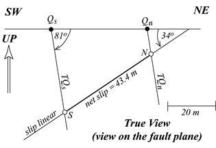
b) true view

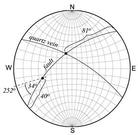
c) stereonet calculation of rakes

Returning to your true view diagram, draw in the quartz vein's contact traces (Fig. 5.4b). Now draw a line representing the slip linear. This line can be drawn at any convenient place on your construction, so long as it crosses both vein-segment traces.

In this case, we already know the rake of the slip line. Had we been given the rake to begin with, instead of the plunge and trend, we would now calculate the plunge and trend of the slip line using the stereonet.

The magnitude of the net slip is the distance between the point S, where the slip linear crosses the trace of the southern contact segment, and the point N, where the slip linear crosses the trace of the northern contact segment. The magnitude of the net slip is 43.4 m.

We obtain the relative movement by comparing the positions of the points S and N and by looking at the orientation of the fault on the map. The northwest side of the fault has gone up and to the northeast with respect to the southern side. (Visualize this motion by using your hands as the two segments of the displaced quartz vein and an imaginary surface between them as the fault.)

Another way of giving relative movement for an inclined fault is to refer to the relative movement of either the hanging wall block or the footwall block. In this case, the hanging wall block has gone up and to the northeast.

Lesson 4: Practice Plus

Do exercise 11, parts (b) and (c) (Marshak & Mitra, pp. 128-129). For (b), pretend that horizontal slickenside lineations occur in the fault zone. For (c), pretend that vertical slickenside lineations were found. Do as much of the question as you can before looking at the solution.

Solutions

Part 1

In structural geology, with a little creativity, the techniques you learn enable you to reduce seemingly complex situations into relatively simple problems. The first challenge in exercise 11 is dealing with the complex collection of faults (the fault zone). You are asked to find the cumulative displacement, which means the total displacement across the entire fault zone.

Start by making this problem look more like other problems you've studied. First, estimate the trend of the fault zone by “eyeballing” the average trend of the faults. The zone appears to trend approximately N23°E. Draw in two lines trending N23°E to bound the fault zone (Fig. 5.5a, below).

In parts (b) and (c), you are given the orientation of the slip line. This means you can solve the problem if you can find the orientation of only one plane that has been displaced by the fault. To find the cumulative displacement across the fault zone, you must be able to determine where this plane intersects the fault line on both the eastern and western sides of the fault zone.

One choice of planes is the southern contact between the Shoo Fly Complex (DOsf) and the lower member of the Sierra Buttes Formation (Dsl). The intersection of the southern DOsf/Dsl contact and the western-most fault (C_w) is visible in the northern part of the map area (Fig. 5.5a). The point of intersection between the southern DOsf/Dsl contact and the eastern-most fault (C_e) is not visible, but you can project the contact under the Tertiary volcanics (Tv) using the strike of Dsl (N29°W, measured from the map symbol) as a guide.

In Figure 5.5b, the essential details have been extracted from the map. You may have noticed that the northwest corner of the map contains two strike and dip symbols for Dsl: one very similar to the southern symbol, and one striking approximately east-west and dipping steeply to the north (Fig. 5.5b). The map gives two strike and dip symbols because the attitude of Dsl changes further to the northwest, where it is folded. In cases such as this, where you must decide which data to use, opt for the data that are closest to the region of interest.

The final step required for the set-up of this problem up is to represent the fault zone as a single pencil line. Do this by “sliding” the sides of the fault zone towards each other in a direction that is perpendicular to the strike of the faults.

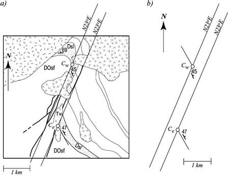
Figure 5.5. Geological map (a) reduced to its essential information (b)

Part 2: Displacement along a Strike-Slip Fault

For part (b) of exercise 11, you are told to assume that the fault is a strike-slip fault with horizontal slickenside lineations. This means that the slip line is oriented horizontally. This assumption does not provide us with the dip of the fault, but in this case the problem can be completed without knowing the dip. Purely strike-slip faults exposed on flat topography are the one case where the net slip can be determined simply by measuring the offset of the contacts directly from the map. Therefore, the cumulative displacement across the fault zone is 2.3 km (Fig. 5.5c, below). The direction of the displacement is along N23°E, and the sense of displacement (the relative motion) is that the western fault block moved northeast relative to the eastern fault block.

Part 3: Displacement on a Purely Dip-Slip Fault

For part (c) of exercise 11, you are told to assume that the fault is purely dip-slip, and that vertical slickenside lineations were found. This means that not only is the slip line oriented vertically, but the fault plane itself is also vertical.

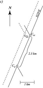
Figure 5.5, continued: (c) simplified problem with measurement of pure strike-slip displacement

Proceed by calculating the rake of the DOsf/Dsl contact on the fault. The dips near C_e and C_w are 47°NE and 45°NE, respectively. These are similar enough that it is reasonable to use the average of the two, 46°NE, as the dip of the contact. To summarize, find the rake of the contact with attitude N29°W, 46°E on the fault with attitude N23°E, 90°. We already know that the slip line is oriented vertically on the fault plane.

Next, draw the true view of the fault as in Figure 5.4b. You should measure a net slip (cumulative displacement) of 1.9 km and find that the western side of the fault moved up relative to the eastern side of the fault.

An important observation to make about this practice problem is that one outcrop pattern works equally well as a strike-slip fault or a dip-slip fault. Without the additional data provided about the slip direction, we would not be able to tell what kind of fault it was. Keep this in mind when you encounter new problems. Treat the fault as though it has a dip-slip component (i.e., draw the true view) unless you have evidence that the fault is purely strike-slip. Laterally offset beds alone are not sufficient proof.

Assignment 5

You should now complete the lab portion of Assignment 5, which you can find in the assignment drop box. Assignment 5 is worth 6% of your final grade (theory portion: 2.5%; lab portion: 3.5%).

After you have completed Assignment 5, please submit this assignment (both theory and lab portions) to your tutor for grading. Please submit your assignment via the appropriate assignment drop box at your online course site. If you are unable to use the assignment drop box, please contact your tutor for an alternative submission method.