Geology 319 Structural Geology: The Architecture of Earth’s Continental Crust

Lab Unit 1

Using Geological Maps: Part 1

Overview

Making geologic observations from a map is an important skill in structural geology. Another important skill is expressing those observations in a way that will help you better understand the overall geologic “theme” of the region. More specifically, the goal may be to use map or field observations to determine what rocks look like beneath the Earth's surface. From there, it is possible to figure out how the rocks got there in the first place and what forces have shaped them since that time. In Lesson 1 you will learn how to use a topographic map to determine the elevation of a region. In Lesson 2 you will learn how to transform the information from the topographic map into a picture of the landscape. In Lesson 3 you will work with a geological map, learning how to read strike and dip from map symbols, how to identify unconformities, and how to identify strata with horizontal or vertical dips. In Lesson 4 you will learn how to add information from a geological map to a topographic profile, creating a picture of what the rocks look like beneath the surface.

Objectives

After working through this lab unit, you should be able to

use a topographic map to
1. make qualitative and quantitative observations about the shape of the Earth's surface.
2. draw a topographic profile along a transect.
use a geologic map to
1. amake general observations about the orientation of geologic units in the map area.
2. draw a geologic cross-section to show what the rocks look like beneath the Earth's surface.

Materials

Basic Methods of Structural Geology by Marshak & Mitra
several sheets of 8½″ × 11″ plain, white paper
protractor
ruler
pencil
eraser
coloured pencils
tape
calculator

Lesson 1: Using Topographic Maps

What Is a Topographic Map?

A topographic map shows the elevation of the Earth's surface. The variations in elevation of a region are generally called its topography, and the difference in elevation between the highest and lowest points is called topographic relief. For example, we would say that the Prairies have a low topographic relief, whereas the Rocky Mountains have a high topographic relief.

A topographic map expresses elevation as contour lines. Contour lines connect points of the same elevation. On page 20 of your Marshak and Mitra textbook, Figures 2-1 and 2-2 show examples of how hills are mapped using contour lines.

Contour lines are spaced at a constant contour interval (often abbreviated CI) that is chosen to conveniently express the changes in elevation. The contour interval is usually written on a topographic map, but you can also find it by simply examining adjacent contours and subtracting one from the other to find the difference between them. (Note: For convenience, not all contour lines on a map are labelled with the elevation. In Fig. 2-1, for example, contour lines are labelled only at every 100 m.)

The contour interval is chosen to present enough contour lines to capture important variations in topography, but not so many that the topographic map is difficult to read. Compare Figures 2-1 and 2-2 again. In Figure 2-1, the topographic relief is low compared to that in Figure 2-2. The topographic range in Figure 2-1b is greater than 160 m, whereas the range in Figure 2-2a is greater than 1400 m. In Figure 2-1b, the topographic variation is adequately expressed with a contour interval of 20 m, whereas in Figure 2-2a, the contour interval is 100 m.

Qualitative and Quantitative Observations from Topographic Maps

We can glean both qualitative (descriptive) information and quantitative information (measurements) from topographic maps.

For example, if you were backpacking in the region shown by Figure 2-2a, and someone in your party became injured, it would be useful to know assess the steepness of the terrane, so you could choose the best route for evacuation. On a topographic map, the topographic contours of steep slopes are spaced more closely together than those on gentle slopes. (Marshak & Mitra, Fig. 2-3, p. 20 illustrates this relationship.) In Figure 2-2a, the contours of the steepest slopes are spaced so closely together that it is not possible to see the individual lines. In the injury scenario above, your party might choose a trail that traverses a region with more widely-spaced contours to evacuate the injured member with less risk of slips, falls, and further injury.

Sometimes, more specific quantitative information is required. For example, the SME Mining Engineering Handbook makes recommendations about the construction of safe and economical mine haulage roads. Among the recommendations are that the roads used by trucks to carry materials to and from mines should be as short as possible (for the sake of convenience), but the grade of their slopes should not overwhelm the engines and braking capacity of heavily loaded trucks. The SME Handbook suggests that an 8% grade (a slope angle of 4.6°) meets this requirement. (Note: The terms grade, slope, true slope, slope angle, and gradient all express steepness, although they do so in slightly different ways.) The engineer in charge of designing a mine haulage road could use a topographic map to calculate how steep the terrane was, which would be useful information in deciding where and how to build the road.

Calculating True Slope

The mine road engineer's first job would be to determine the slope of the terrane that the road would have to cut across. If Figure 1.1a (labs) is a topographic map of the mine region, and the mine is at the top of the hill at point A, how steep would a road be that travelled directly up the hill (that is, along a path that intersects the contour lines at 90°) along the traverse B-A?

Figure 1.1b (labs) shows a diagram of the problem drawn on the same scale as 1.1a. The advantage of drawing the diagram to the same scale is that you can find the answer by measureing directly from the scale drawing. This technique is called descriptive geometry. You will see many more examples of descriptive geometry throughout this course.

In Figure 1.1b, the line A-B′ represents the hillside (the surface the trucks will drive on); A-B represents the run (the horizontal distance travelled); and B-B′ represents the vertical distance travelled, called the rise. The line A-B is at 90° to the line B-B′. Note that B is not located on a topographic contour but between two contours. The elevation for B′ in Figure 1.1b was determined by interpolation. In other words, because B is situated approximately halfway between the 200 m and 100 m contours in Figure 1.1a, we estimate that the elevation at B′ is 150 m. You can measure the true slope angle, Ø, with your protractor. The true slope angle here is 34°.

Note that the true slope angle could also be determined by trigonometry instead of by descriptive geometry, because triangle ABB′ is a right-angle triangle:

$\begin{aligned} \tan φ = & \frac{rise}{run} \\ φ = & \tan^{- 1} (\frac{rise}{run}) \\ = & \tan^{- 1} (\frac{350 m}{512.5 m}) \\ φ = & 34 ° \end{aligned}$

The same information can be expressed as a true slope gradient in units of m/km:

$slope gradient = \frac{350 m}{512.5 m} \times \frac{1000 m}{1 km} = 683 \frac{m}{km}$

The information can also be expressed as a grade in per cent:

$grade = \frac{350 m}{512.5 m} \times 100 % = 68.3 %$

Fig L1.1

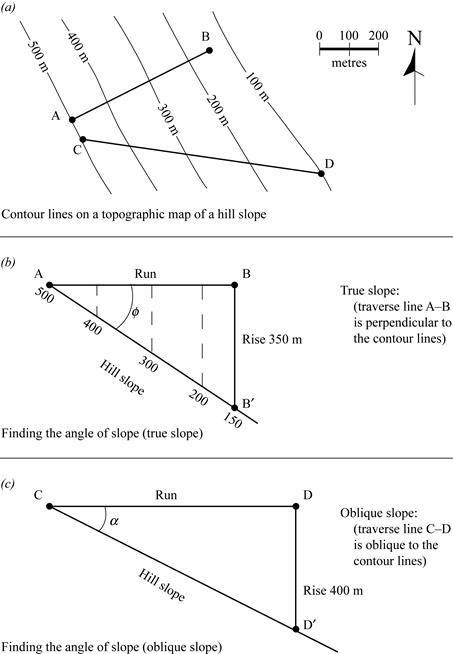
Figure 1.1. Calculation of topographic slope using descriptive geometry

Expressed as a grade, the hillside is clearly far too steep for the mine road to be constructed along the traverse A-B. To reduce the grade, the road will have to be built along an oblique slope. The slope of the line C-D in Figure 1.1a is an oblique slope, because the transect C-D does not intersect the contour lines at right angles. Any transect that is not perpendicular to the contour lines will have a slope less than the true slope.

Figure 1.1c illustrates the descriptive geometry solution for the oblique slope angle, α. The solution works the same way as the true slope solution, and the trigonometric solution can apply as well.

So, if the mine road must go from the 500 m contour line to the 100 m contour line directly downhill from A, we can work backward from the 8% grade requirement. We can draw a triangle like CDD′, and determine the run that would be needed over a rise of 400 m.

To have a grade of 8%, there must be 100 m of run for every 8 m of rise.

$100 m \times \frac{400 m}{8 m} = 5000 m$

This means that if the mine road must rise a distance of 400 m, the run will need to be 5000 m. The road must be 5 km long! The best way to accomplish this without having to drive a long distance away from the mine is to fold the road into a series of switchbacks.

Reading Assignment

Read Marshak & Mitra: “2-1. Introduction” and “2-2. Elements of Contour Maps” (pp. 19-23). Pay special attention to the section, “General Constraints on Contour Maps.”

Lesson 2: Drawing Topographic Profiles

While it is possible to imagine what a terrane looks like from a topographic map, it is sometimes important to know what the terrane looks like in more detail along a particular transect. To achieve this, we draw a topographic profile. A topographic profile is what you would see if you could cut vertically into the Earth along a transect and then viewed the cut from the side.

Figure 2-6 (Marshak & Mitra, p. 22) shows four examples of topographic maps and topographic profiles drawn along the transect X-X′. For the moment, focus on the shapes of the profiles (i.e., the outline of the top of the shape), and notice how the different groupings of contour lines on the maps produce different shapes.

Drawing a topographic profile is not difficult, but it is important to pay attention to the details, because a topographic profile is often the starting point for more complex analyses.

Figure 1.2 (labs) illustrates the process of drawing a topographic profile

Fig L1.2

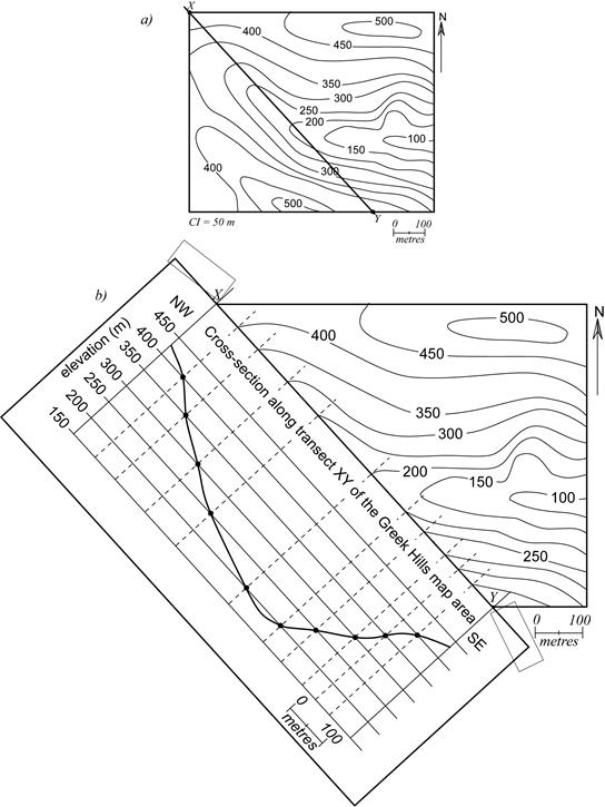
Figure 1.2. How to draw a topographic profile

The first step is to draw a transect where the profile is to be constructed. In Figure 1.2a, the transect is between points X and Y.
The next step (Figure 1.2b) is to take a piece of blank paper, align it with the transect, and secure it to the map with tape.
Draw a box with horizontal lines representing the elevations along the transect. Go one contour interval above the highest elevation along the transect and one contour interval below the lowest elevation. Make the spaces between the horizontal lines to the same scale as the map.
Now it is time to mark elevations in the box. Along the top of your page, mark every point where the transect intersects a contour line. With a faint pencil line, extend a line from the transect down into the box (dashed lines in Figure 1.2b). Mark the point where the dashed line intersects the appropriate elevation. For example, where the transect intersects the 400 m contour line, there is a point marked at the intersection of the dashed line and the horizontal line, representing the 400 m elevation.
When you have all of the elevations plotted in the box, you can connect the dots. Try to connect them with a smooth curve. Where two or more points remain at the same elevation, your line will change direction. For example, the transect intersects the 200 m contour line twice in Figure 1.2b. In the topographic profile moving from left to right, this is where the topography changes from going downhill to going uphill. We don't know how far beneath the 200 m contour line the topography should go, but we do know that it should not touch the 150 m contour line. At the ends of the topographic profile, extend the line to approximate the change in topography. Do not end the line abruptly if the last point does not coincide with the end of the transect.
You should always include a title for a topographic profile. You should always mark the orientation at either end, and include a scale.

Topographic Profiles and Vertical Exaggeration

If the topographic relief of a region is low, a topographic profile drawn using a map scale may be impractical. The map scale may be too small to reveal useful information for a topographic profile. In such a case, the profile can be drawn with vertical exaggeration. Vertical exaggeration is a way of stretching the profile vertically by using a scale that is larger than the horizontal scale from the map.

For example, if you wanted to draw a topographic profile from a map with a scale of 1:50,000 and a 50 m contour interval, then the horizontal lines of your profile would have to be very close together. The scale of 1:50,000 means the same as 1 mm = 50,000 mm, or 1 mm = 50 m. Therefore, the horizontal lines would be only 1 mm apart. Plotting the profile would be much easier if the horizontal lines were 1 cm apart. Using a spacing of 1 cm would give you a scale of 1 cm = 50 m, which is the same as 1 cm = 5000 cm, or 1:5000.

When you use a vertical scale that is different from the horizontal scale, it is common practice to indicate the difference between the scales by calculating the vertical exaggeration (VE):

$VE = \frac{vertical scale}{map scale} = \begin{matrix} \underline{\frac{1}{5000}} \\ \frac{1}{50000} \end{matrix} = \frac{1}{5000} \times \frac{50000}{1} = \frac{50000}{5000} = 10$

On your topographic profile you would report that you used a vertical exaggeration of 10 times.

Lesson 3: Understanding Geologic Maps

A geologic map shows the distribution of rock beds on the surface of the Earth. Geologic maps are often combined with topographic maps.

The pattern made by rocks on Earth's surface depends on the orientation of the beds and the topography. Topographic variation often causes the exposure of rock beds to appear in complex patterns, even when the shape of the bed itself is not complicated. In this lesson you will learn how to draw a geologic cross-section. You will then be able to translate complex surface patterns into a picture of the rocks beneath the Earth's surface. Before we can do that, however, you must first learn how the orientation of planar geological structures is described.

Strike and Dip

Reading Assignment

Read Marshak & Mitra: “1-1. Introduction,” “1-2. Reference Frame,” and “1-3. Attitudes of Planes” (pp. 3-7)

In geometrical terms, all structures can be represented as planes or lines. The orientation of a plane or line in three-dimensional space is referred to as its attitude. In this lab unit, we will focus on the orientation of planar structures.

A planar structure, such as a rock bed or a fault plane, can be described by two measurements. One measurement, the dip, describes the tilt of the plane. Dip is measured down from horizontal (Figure 1.3 below). A horizontal plane would have a dip of 0°, and a vertical plane would have a dip of 90°.

Fig L1.3

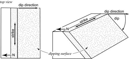
Figure 1.3. Describing the attitude of a planar structure using strike and dip

The other measurement gives the orientation of a plane in a geographic coordinate system. There are two ways to do this. One is to specify the dip direction, or the direction in which the plane tilts downhill (i.e., the direction water would flow down the plane). It is more common, however, to specify the strike. The strike of a plane is the geographic orientation of a horizontal line that intersects the plane. Strike is always perpendicular to the dip direction.

There are two systems used to report geographic orientations: the quadrant convention, and the azimuthal convention. Marshak and Mitra illustrate these in Figure 1-5 (p. 5). In the quadrant convention, the geographic direction is given by specifying the angle away from either north or south. For example, if you were travelling NE, you would report your direction as N45°E. In other words, start from north, and rotate 45° to the east.

With the azimuthal convention, geographic space is divided into 360°, and all directions are reported using three digits. For example, NE would be 045°.

Reporting Strike and Dip

The attitude of a plane is most commonly specified by listing the strike direction followed by the dip angle and a general dip direction. In Figure 1-3 above, for example, the speckled bed is dipping at an angle of 50° to the south, and is striking east-west. Each of the following are valid ways to specify the strike and dip of the speckled bed:

Quadrant convention		Azimuthal convention
N90°E, 50°S	S90°E, 50°S	090°, 50°S
N90°W	S90°W	270°, 50°S
50°S	50°S

Strike and Dip on a Geological Map

A special symbol is used to indicate strike and dip on geological maps:

Strike and dip symbol

The long line is oriented along the strike direction. On a map, you can get the strike from this symbol by measuring the direction of the long line relative to north. The short line indicates the dip direction, and the dip angle is written next to the symbol. Figure 1.4 (Greek Hills Map Area) shows a geological map with the topographic map from Figure 1.2 superimposed. (These two kinds of maps are often combined.) In Figure 1.4, bed F has a strike and dip symbol indicating that it has an attitude of N41°E, 17°NW.

The attitude N41°E, 17°NW applies to beds C, D, E, and G as well, but not to the igneous intrusion, or to beds A and B. The igneous intrusion represents the special case of a bed with a vertical dip. You can tell the bed is vertical because both contacts (outer surfaces) of the bed appear as straight lines, even in the presence of topography. The strike of a vertical bed can be measured directly from the map. The igneous intrusion has an attitude of N20°E, 90°. Note that a general dip direction is not required when the dip is vertical.

Beds A and B are another special case. If you look carefully at the map, you will see that the contacts of beds C through G intersect the contour lines. This is to be expected if the beds are dipping. However, the contacts of beds A and B do not intersect the contour lines. This means that they are horizontal (or very nearly so), with a dip of 0°. Strike is not specified for horizontal beds, because the intersection of a horizontal plane with another horizontal plane contains an infinite number of horizontal lines in an infinite number of directions.

The heavy black line along the lower contact of bed B marks an important interval called an angular unconformity. (Unconformities are discussed in detail in Unit 2 of the Study Guide.) In short, the unconformity is a surface resulting from erosion after beds C through G were deposited and then tilted by 17°. It is called an angular unconformity because it, and beds A and B above it, are not parallel to beds C through G (Fig. 1.4).

Fig L1.4

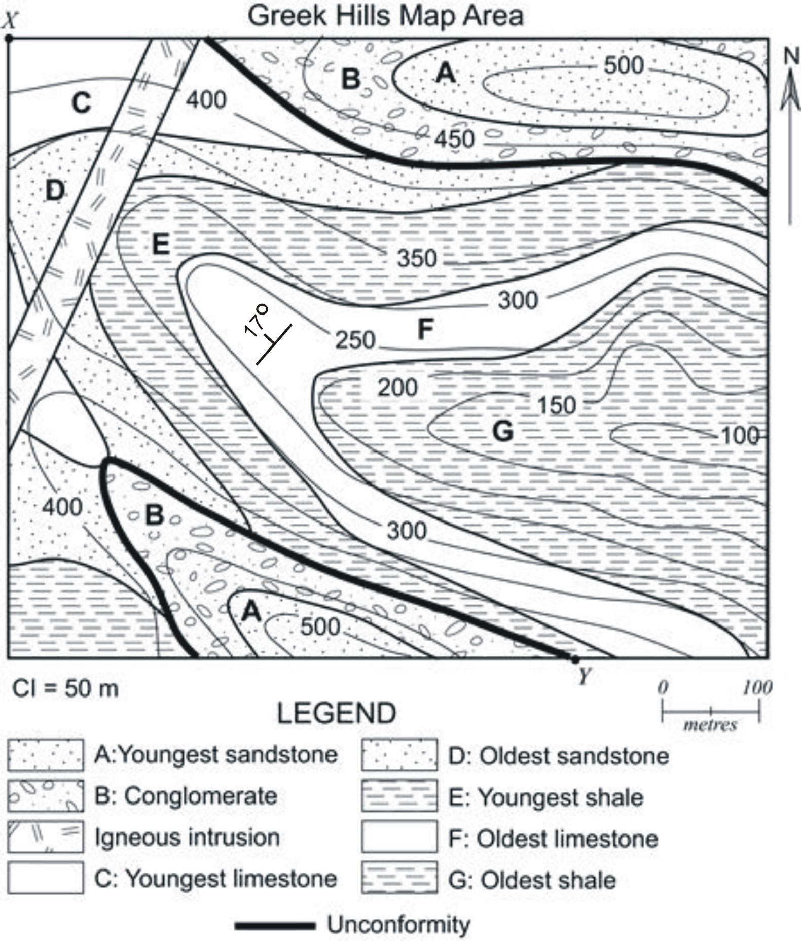
Figure 1.4. Geologic map of the Greek Hills Area

Lesson 4: Drawing Geological Cross-Sections

Like topographic profiles, geological cross-sections are drawn along a transect. As an example, we will use the transect X-Y as before. Transects are chosen to best highlight the geological features of interest, but most often a transect is chosen such that it runs parallel to the dip direction. This is because viewing dipping beds in a plane oblique to the dip direction makes them appear to have less of a dip than they actually do. To construct a cross-section that accurately represents the appearance of the beds, would require calculating what the smaller dip angle would be. For now, we will concern ourselves only with cross-sections parallel to the dip direction.

The first step of drawing a geological cross-section is to draw the topographic profile along the transect (Fig. 1.2b, labs). Note that the dip angle must be adjusted if the topographic profile is drawn with vertical exaggeration. We will not use vertical exaggeration here.

Fig L1.5

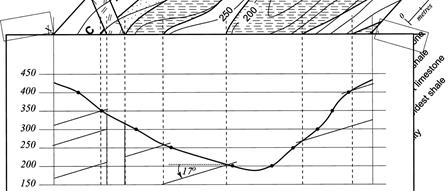
Figure 1.5. Drawing a geological cross-section

The next step is to mark and draw in the lithologic contacts. Lithologic contacts are marked in the same way that topographic contours were marked: mark every point where the transect intersects a lithologic contact along the top of your page (see Fig. 1.5 above). Extend a line from the mark down to the topographic profile (Fig. 1.5, dashed lines). Where the line intersects the topographic profile, draw the contact by measuring the dip angle down from horizontal. Note that the igneous intrusion cross-cuts (cuts through) the sedimentary layers on the map, so it should also cut through the sedimentary layers in the cross-section.

The completed cross-section is shown in Figure 1.6. There are a number of important details to note:

Where both contacts are present, beds have uniform thickness.
The lower contact of bed G is drawn as a dashed line with question marks. This indicates that we do not know the thickness of bed G.
The beds get younger in the dip direction.
When finished, your cross-section should have LOTS:
1. Legend: List the rocks that appear in the cross-section from youngest to oldest. Do not include rocks that are in the map area but that are not in the cross-section.
2. Orientation: Indicate the general orientation of the cross-section by labelling it at either end. Do not use a north arrow. North arrows are reserved for maps.
3. Title
4. Scale

Fig L1.6

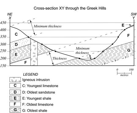
Figure 1.6. Completed geological cross-section

You may have noticed that patterns have been used in Figures 1.4 and 1.6 to indicate the composition of a particular rock. Alphabet letters have been used on the geological map and the cross-section to distinguish between strata of different ages, but that have the same composition. Although it is common for the beds in geological maps and cross-sections to have short labels that reflect their age and the name given to the rock formation, colour (or patterns, if black-and-white) is the usual way to distinguish between beds. You can see this by examining your map of Whiterabbit Creek (see your course package) and the accompanying geological cross-sections.

Measuring the True Thickness of Beds

Dipping beds: If both contacts of a bed are present, the true thickness, or stratigraphic thickness, of a bed can be determined. The true thickness is the distance between the upper and lower contacts of a bed along a line that is perpendicular to the contacts. For example, the true thickness of bed F in Figure 1.6 (labs) is 92 m.

For beds where only one contact is known (e.g., beds C and G), you can estimate the minimum thickness. For bed C, the thickness is >104 m; for G, >35 m.

Horizontal beds: The same procedure works for horizontal beds. However, the thickness of horizontal beds can also be measured directly from the map: determine the elevation of the upper and lower contacts, then subtract to get the difference.

For example, the lower contact of bed B (Figure 1.4, labs) is approximately halfway between the 400 m and 450 m contour lines, so the elevation of the contact is approximately 425 m. The upper contact of bed B is approximately halfway between the 450 m and 500 m contour lines, so the elevation of the upper contact is approximately 475 m. Therefore, the thickness of bed B is 475 m minus 425 m = 50 m.

In the case of bed A, only the lower contact is present, so we can only estimate the minimum thickness. From the previous example, we know the lower contact of bed A has an elevation of 475 m. The maximum elevation of A is greater than 500 m, but less than 550 m. Unfortunately, we don't have a 550 m contour line to help us estimate where (between 500 m and 550 m) the elevation falls, so we will err on the conservative side and use 500 m. (After all, the upper contact could have had an elevation of 501 m, or it could have been 549.5 m. We just don't know.) Therefore, we estimate the thickness of bed A at >25 m.

Vertical beds: The true thickness of a vertical bed can also be measured from a map, as long as it is measured perpendicular to the contacts of the bed. The igneous intrusion in Figure 1.4 (labs) has a thickness of 44 m. Note that if you try to measure the thickness of the igneous intrusion in the cross-section, you will get a result of 49 m. The cross-section does not give the correct thickness because the transect of the cross-section does not intersect the igneous intrusion at 90° to the contacts of the intrusion. You can see this in Figure 1.5, or by drawing in the line XY in Figure 1.4. It is possible to measure the correct thickness of a vertical bed in a cross-section if the transect of the cross-section runs perpendicular to the strike of the igneous intrusion.

Assignment 1

You should now complete the lab portion of Assignment 1, which you can find in the assignment drop box. Assignment 1 is worth 6% of your final grade (theory portion: 2.5%; lab portion: 3.5%).

After you have completed Assignment 1, please submit this assignment (both theory and lab portions) to your tutor for grading. Please submit your assignment via the appropriate assignment drop box at your online course site. If you are unable to use the assignment drop box, please contact your tutor for an alternative submission method.