Geology 319 Structural Geology: The Architecture of Earth’s Continental Crust
Lab Unit 6
Fold Orientation: Structural Clues
Overview
Folds may occur on a variety of scales. If a fold is small enough for you to see the closure of the fold, you can measure its orientation directly using a geological compass. You will learn how to do this in Lab Unit 7. However, if a fold is large, you may only see small parts of it. In this case, a direct measure of its orientation is not possible. Fortunately, by collecting data from a number of small exposures, it is possible to determine the orientation of the fold. Lesson 1 summarizes the issues involved in using the stereonet as a statistical tool, and describes what information about folds can be determined using a stereonet. Lesson 2 describes the use of the stereonet and data about bedding plane orientations to determine the orientation of the fold axis and axial plane. Lesson 3 describes the use of cleavage data for determining these characteristics. Lesson 4 covers the methods for representing folds on geologic maps.
Objectives
After working through this lab unit, you should be able to
- use the orientation of beds in the limbs of a fold to determine the attitude of the fold axis and the axial plane of the fold.
- use the orientation of cleavage planes generated by folding to determine the attitude of the axial plane of a fold.
- identify a fold on a geological map by clues such as outcrop patterns and map symbols.
- use map symbols to indicate the presence of a fold.
Note: You will require a firm understanding of Study Guide Unit 5 to do this lab.
Materials
- Basic Methods of Structural Geology by Marshak & Mitra
- Structural Geology of Rocks and Regions by Davis, Reynolds, & Kluth
- stereonet
- several sheets of 8½″ × 11″ plain, white paper
- several sheets of 8½″ × 11″ tracing paper
- protractor
- ruler
- pencil
- eraser
- coloured pencils
Lesson 1: Using the Stereonet as a Statistical Tool
Before we begin to analyze folds, let's break down the jobs involved. There are actually two sets of skills to learn for this lab. It makes sense to briefly point these out because it is usually easier to understand how to do a task if you understand why the steps are necessary.
Task 1: Using the Stereonet as a Statistical Tool
The analysis of large faults requires the collection of data from a number of small outcrops. Depending on what properties you are trying to measure, collecting more data has certain advantages:
- The more data you collect, the better your chances of capturing the necessary range of data to make your conclusions reliable. In some cases, if you do not have data representative of all of the different circumstances that exist, the data, though correct, will lead you to make the wrong interpretation. This kind of error is called a sampling bias. It means that your result is a consequence of how you collected your data, not the actual circumstances you intended to measure.
- The more data you collect, the better your chances of outweighing anomalous data with data more representative of the situation. For example, consider measuring the strike and dip of a bed in the field. If you make only one measurement at the first outcrop you encounter, it may turn out that you sampled a site where the attitude of the bed differs on a small scale from its overall attitude. If you made a second measurement at another outcrop and got a result different from the first, you have no way of knowing which of your two measurements is correct. If you make a number of measurements, all of which will likely differ to varying degrees, you can best decide what strike and dip the evidence seems to support most.
While having abundant data can be beneficial, you must also have a convenient and effective way to represent and interpret the data. As you saw in Lab Unit 4, the stereonet is just the tool for the job. Return to Lab Unit 4 if you need to review the semi-statistical use of the stereonet.
Task 2: Interpreting the Data
The new material introduced in this lab concerns how to use the results of your semi‑statistical analysis to determine the orientation of a fold.
Reading Assignment
- Read Davis, Reynolds, & Kluth: “Stereographic Determination of Fold Orientations” (pp. 366-368)
- Read Marshak & Mitra: “8-5. Analysis of Folding with an Equal-Area Net” (pp. 157-159)
Your goal for these readings is to learn the following:
- What fold characteristics can you determine from a beta (β) diagram?
- What fold characteristics can you determine from a pi (π) diagram?
- Why do Marshak and Mitra say that “A plot of β-axes is not generally the best way to represent attitude measurements on a fold”?
- Define bisecting surface and interlimb angle. In your notes, make a sketch to illustrate these terms.
- What simplifying premise is made about the bisecting surface of a fold?
Lesson 2: Use of the β and π Methods to Determine Fold Orientation
The orientation of bedding measured at different locations across a fold can be used to determine the attitude of the fold axis and of the axial plane. The readings have introduced these methods. In this section, we will use the following strike and dip measurements of folded beds to illustrate the methods:
110°/40°SW 150°/45°SW
080°/40°SE 040°/50°SE
005°/70°SE 050°/45°SE
132°/60°SW
The β-diagram (Fig. 6.1)
On a new overlay, plot the fold limb orientations as planes.
Mark each intersection between planes with a point. If more than two planes intersect at a single location, draw a circle around the point for each additional plane.
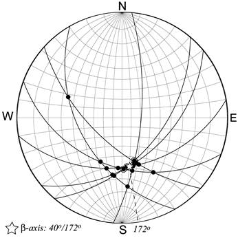
Figure 6.1. β-diagram
Mark the centre of density of the point distribution. In Figure 6.1 (labs), the centre of density is marked with a star. Use the circles to help you to account for the extra “weight” of intersections of more than two planes. One way to think about the weight of points is to imagine each intersection as a small magnet. Where more than two planes intersect, there is an additional magnet for each additional plane. Now imagine that you have a small iron sphere suspended on a string. If you were to hold the sphere just above the centre of the cluster of magnets, each magnet would exert a force on the sphere; magnets located closer together would have a stronger pull on the sphere than a single magnet by itself. Therefore, the suspend sphere might be pulled more to one side than another. The centre of density of the point distribution is the point above which the sphere would come to rest.
The centre of density on a β-diagram is referred to as a β-axis. It is an estimate of the orientation of the fold axis. In our example, the β-axis has an orientation of 40°/172°.
The π-diagram (Fig. 6.2)
On a new overlay, plot the poles to the fold limb orientations.
Rotate the overlay until you find the great circle that best fits the set of poles. If the fold measurements are correct, your plotting is correct, and the fold is perfectly cylindrical, then all of the poles should fall on a single great circle. In this example, however, this is not the case, so a great circle has been chosen using the following criteria:
- Many of the poles fall on the great circle, or very close to the great circle.
- For poles that do not fall on the great circle, an attempt is made to distribute them as evenly as possible on either side of the great circle.
The great circle you choose to fit the poles is called the π-circle. Find the pole to the π-circle. This is called the π-axis. The π-axis for this example is oriented 40°/175°. The π-axis, like the β-axis, is an estimate of the fold axis. Under ideal circumstances, the β-axis you calculate should be the same as the π-axis. This unusual, however, because it is much more difficult to judge the centre of density of a point cluster than it is to fit a curve to a set of points.
The π-diagram can also be used to estimate the orientation of the axial plane. To do this, we use the angle between the fold limbs, called the interlimb angle. The interlimb angle can be estimated from the spread of the poles along the π-circle. In Figure 6.2, the interlimb angle measured through the poles is 105°. (You can measure this by rotating your stereonet until the π-circle lies on a great circle, and then counting off the distance.) Note, however, that there are actually two possible interlimb angles: The other is 75°. To decide which interlimb angle to use requires that you have some additional knowledge about the shape of the fold. If the fold is tightly closed and has an interlimb angle of less than 90°, then you would use 75°. If the fold is less tightly closed, and has an interlimb angle greater than 90°, then you would use 105°.
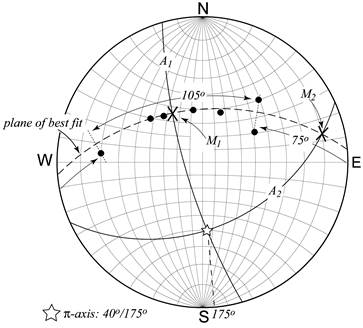
Figure 6.2. π-diagram
Regardless of which interlimb angle you use, the procedure is the same. First, mark the midpoint (x) of the interlimb angle. Next, rotate your overlay until the midpoint and the π-axis lie on the same great circle, and trace the great circle to find the limb bisectrix, the plane that lies exactly between the limbs of the fold (as represented by your data). The limb bisectrix is an approximation of the axial plane.
If we had independent information that the fold was not tightly closed, then we would choose the great circle connecting the midpoint of the 105° angle (M1) and the π-axis. The orientation of the axial plane (A1) would be 164°/76°W. This fold could be described as moderately plunging and steeply inclined.
If we knew that the fold was tightly closed, then we would choose the great circle connecting M2 and the π-axis. The orientation of the axial plane (A2) would be 066°/42°S. This fold could be described as moderately plunging and steeply inclined.
Lesson 3: Using Cleavage to Determine Fold Orientation
In Unit 5, we learned that folded rocks often develop a planar fabric in response to deformation and metamorphism. This planar fabric is called cleavage, and it forms perpendicular to the direction in which the rocks have been flattened. Cleavage is statistically parallel to the axial planes of folds that formed during the same deformation event, even though it commonly refracts or fans away from the hinge of the fold. The general parallelism of cleavage made from measurements across a fold or from a series of related folds provides one of the best ways of analyzing fold orientation (Fig. 6.3a-e).
A π-diagram of cleavage made from measurements across a fold or across a series of related folds will display a cluster of points whose centre of density will closely approximate the pole to the axial plane (or average axial plane). Figure 6.3a and b show an inclined axial plane and average axial-planar cleavage (S1) dipping steeply to the southeast. This procedure generally works best when it is possible to use cleavage measurements entirely from the hinge zone.
If cleavage is parallel to the axial plane (and the folds are cylindrical), then just as the axial plane intersects the folded surface along the hinge line, the cleavage intersects the folded surface parallel to the hinge line (e.g., Fig. 6.3a, below).
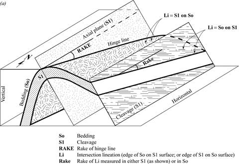
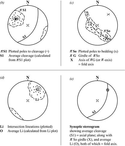
Figure 6.3. Inclined plunging fold with axial planar cleavage
Figure 6.3a shows a cleavage surface (cleavage S1) that is parallel to the axial plane. On this surface, the trace of bedding (So) forms a line with a rake angle (rake) that is equal to the rake of the hinge line in the axial plane (RAKE).
The intersection between cleavage and a folded surface (such as bedding) forms an intersection lineation (Li) that can be seen on either surface. On cleavage surfaces exposed by erosion (or broken open by geological hammer), traces of transected bedding may be displayed (So and S1). Intersection lineations across a fold or series of related folds are never perfectly parallel to each other because of variations in attitude of cleavage, such as fanned cleavage, and lack of perfectly cylindrical folding.
The orientation of intersection lineations can be obtained by
- measuring the rake of Li,
- measuring the rake of Li in S1,
- measuring the plunge of Li, or
- measuring the attitudes of So and S1, and then using the stereonet to calculate any of the above three values.
Note: the average bedding/cleavage intersection for a cylindrical fold will be parallel to the average hinge line (and the fold axis).
Figure 6.3d shows a number of Li plotted for a fold like that in Figure 6.3a. Here the fold plunges gently to the northeast. Compare this result with that obtained from a π-So diagram (Fig. 6.3c).
Figure 6.3e is a synoptic stereogram. It summarizes the fold orientation data derived from the three previous analytical diagrams. Note the coincidence of the average Li and the π-axis, both of which yield the fold axis.
In many folded and cleaved rocks, there is considerable scatter in the orientations of the various structures, making it necessary to make dozens or even hundreds of measurements. Even then, we might not obtain a perfect matching of S1, Li, and the π-axis.
Lesson 4: Representing Folds on Geologic Maps
A fold is represented on a geologic map by drawing a line along the outcrop trace of its axial plane (its axial trace) and adding symbols to indicate several of the fold's attributes. The axial trace is generally determined by drawing a line connecting successive fold noses along the fold. A fold nose is the location on the ground where the trace of the folded surface changes orientation most rapidly (i.e., it has the tightest curvature).
Reading Assignment
- Marshak & Mitra: “Representation of Folds on a Map” (pp. 223-226)
Assignment 6
You should now complete the lab portion of Assignment 6, which you can find in the assignment drop box. Assignment 6 is worth 6% of your final grade (theory portion: 2.5%; lab portion: 3.5%).
After you have completed Assignment 6, please submit this assignment (both theory and lab portions) to your tutor for grading. Please submit your assignment via the appropriate assignment drop box at your online course site. If you are unable to use the assignment drop box, please contact your tutor for an alternative submission method.
Preparation for Lab Unit 7
Lab Unit 7 requires a lab kit that you must borrow from the AU Library. You may wish to order this lab kit now, so that you have it in hand when you are ready to work on Lab Unit 7. You can find instructions for requesting materials from the Library in the Student Manual.