Geology 319 Structural Geology: The Architecture of Earth’s Continental Crust

Lab Unit 7

Introduction to the Geological Compass

Overview

In this unit, you will learn how to measure the orientation of geological structures using a geological compass. Lesson 1 describes the theory behind the magnetic compass, including the meaning of magnetic north and magnetic declination. Lesson 2 introduces the Silva Ranger compass, followed by Lesson 3, where you will learn how to measure strike and dip with the compass; and Lesson 4, where you will learn how to measure plunge and trend with the compass. Lesson 5 covers the techniques for measuring the orientation of a small fold (i.e., a fold that is completely visible).

Objectives

After working through this lab unit, you should be able to

1. set your compass to the appropriate magnetic declination.
2. measure the strike and dip of a planar surface.
3. measure the plunge and trend of a line, and measure the rake of the line in a plane.
4. identify the axial plane of a fold on a fold model, and measure the orientation of the axial plane.
5. identify the hinge of a fold on a fold model, and measure the plunge and trend of the fold axis.
6. measure fold limb orientations and use β- and π-diagrams to determine fold orientation indirectly.

Materials

• GEOL 319 Lab Kit (ordered from the AU Library)
• Basic Methods of Structural Geology by Marshak & Mitra
• Structural Geology of Rocks and Regions by Davis, Reynolds, & Kluth
• stereonet
• several sheets of 8½″ × 11″ tracing paper
• protractor
• ruler
• pencil
• eraser

Lesson 1: Magnetic North

Reading Assignment

• Marshak & Mitra: “Magnetic Declination” (p. 10)

Lesson 1 explains that your compass works by aligning itself along the Earth's magnetic field lines. The magnetic field lines represent the magnetic force generated by convection within the Earth's iron-rich liquid core and by Earth rotating on its axis. Magnetic field lines exit the Earth's south magnetic pole and enter the Earth's north magnetic pole (Fig. 1-16, Marshak & Mitra, p. 10). This causes the magnetic field lines to be much the same as if a simple bar magnet were buried at the centre of the Earth.

Earth's magnetic field changes in a number of ways through time: it varies in strength on the scale of centuries, and approximately every 500,000 years or so, it does a flip, or magnetic reversal, so that your compass needle would point south instead of north. Earth's magnetic field also shifts orientation, so that magnetic poles do not stay in the same position relative to the Earth's axis of spin (its geographic poles). At present, magnetic north is thought to be moving northwest at 40 km per year. Figure 7.1 shows the positions of magnetic north from 1831 to the most recent survey in 2001 (stars), as well as estimated positions of magnetic north between 1600 and 1860, as it wandered through the Canadian Arctic Archipelago. In 2001, the magnetic north pole was approximately 970 km south of true north.

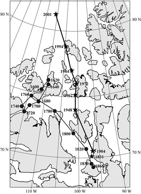
Figure 7.1. Surveyed position of magnetic north (stars), and calculated positions of magnetic north in the past (circles)

In summary:

• Your compass points to magnetic north, not true (or geographic) north.
• The position of magnetic north changes with time.

In geology, as in land surveying, directions are always measured relative to true north, so compensation must be made for the difference between true north and magnetic north. If city planners used magnetic north instead of true north to lay out the streets for new developments, city streets in newer areas would be built on a curve compared to earlier developments, as magnetic north moved!

The difference between magnetic north and true north is described in terms of magnetic declination. Magnetic declination indicates the angle between magnetic north and true north and whether magnetic north is east or west of true north. The magnetic declination at Inuvik, for example, is 26° 7′ E, meaning that if you went to Inuvik and looked at your compass, it would point 26° 7′ eastward of true north.

Source: https://www.ngdc.noaa.gov/geomag/WMM/DoDWMM.shtml

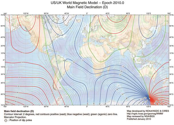
Figure 7.2. Map of global magnetic declination

Figure 7.2 is a map of much of the Earth's surface that shows lines connecting places with equal magnetic declination (magnetic declination contour lines). Note that negative values indicate westward declination. Maps such as this can be used to estimate the declination for a particular location at which geological investigations are taking place. Detailed maps of small parts of the Earth's surface are also available through the geological or land survey branches of most of the world's governments.

There are also online resources that permit the calculation of magnetic declination for a specific location by name or by specifying latitude and longitude. One such resource is provided by the NOAA (National Oceanographic and Atmospheric Administration) in the United States and their National Geophysical Data Centre (www.ngdc.noaa.gov). This World Magnetic Model (WMM) resource was used to estimate the declination and annual change in declination (reflecting the changing position of magnetic north) in 2010 for a number of Canadian cities (Table 7.1).

* Declination is shown in degrees and minutes. There are 60 minutes in one degree.

Table 7.1. Magnetic declination for some Canadian cities

In the next section, you will learn how to adjust your compass for magnetic declination.

Lesson 2: Meet the Silva Ranger 15TD-CL

There are many different types of geological compasses in use around the world. The compass shown in Figure 1-14 (Marshak & Mitra, p. 9) is the Brunton compass, recognized as a precision compass widely used by those who need to make accurate measurements of degrees and angles in the field. However, other compasses can also do the job (with a smaller initial investment). In this course you will learn to use the Silva Ranger, which you can find in the lab kit that you borrowed from the AU Library. At the time of this writing, the model you will use (15TD-CL) is no longer sold, but the Silva Ranger 515 has very similar features. Brunton also sells a line of similar compasses.

The Silva Ranger consists of two main components common to all geological compasses:

1. a magnetic compass for measuring horizontal angles, and
2. an inclinometer for measuring vertical angles.

Reading Assignment

• Read Davis, Reynolds, & Kluth: “E. Measuring the Orientations of Structures” (pp. 711-717)

  Note: Marshak & Mitra also cover the basic use of the geological compass (pp. 8-14).

Getting to Know the Silva Compass

The following discussion assumes that you have not used a compass before.

To open your Silva, press the end of the clip down while lifting up on the clip-end of the black mirror case. Compare your Silva with that shown in Figure 7.3, and identify the following parts:

1. Magnetic needle: The red-tipped end of the needle points to magnetic north. The needle is housed in an oil-filled chamber. The oil slows the motion of the needle to make it less sensitive to unintentional motion as you try to make measurements.
2. Calibrated direction ring: This ring is used to measure horizontal directions. It is made of black plastic and is marked off in two-degree increments from 000 to 360. (Note: 000 is in the same place as 360, but only 360 is marked on the ring.) Turn the direction ring back and forth a few times. You will see that the entire compass chamber moves with it, but the magnetic needle stays more or less stationary.
3. The base of the compass chamber consists of two thin, clear, plastic plates. One is marked with an outline arrow. The other is a calibrated plate. It is marked with lines and numbers from 0 to 90 degrees in both directions away from 0.
4. The compass chamber also contains an inclinometer arm. It consists of a red arrow printed on clear plastic, which swings freely when you shake the compass. It is used to measure vertical angles.
5. There is a small brass screw near the 040° position on the direction ring. It is used to adjust for local magnetic declination. Use the tool at the end of the neck cord to carefully turn the screw by a small amount. As you turn the screw, notice that the outline arrow plate inside the compass chamber moves past the calibrated plate.

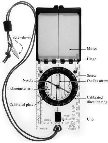
Figure 7.3. Silva Ranger 15TD-CL geological compass

Adjusting for Magnetic Declination and Measuring Bearings

The aim of the following discussion is to acquaint you with how the compass works and to give you some practice with it. We will work with four different magnetic declinations: 0°, 15°E, 20°W, and the declination at your location. For the first three declinations, compare your compass to the images (figures) of the compass settings (below). Some of the images are accompanied by a vector diagram to help you understand the relative positions of true north (Tn), magnetic north (Mn), and the bearing in question.

When you work through the exercises provided, be sure to avoid “mixed signals” from nearby iron or steel objects, or sources of electromagnetic fields such as power lines. Even a steel belt buckle can interfere with your compass. If possible, do these exercises outdoors and well away from sources of interference. If you must do these exercises indoors, try to stand in the centre of the room and as far away from steel objects and electrical appliances as possible.

Case 1: 0° Declination

Set your compass to 0° declination by turning the small brass screw until the centre mark of the blunt end of the outline arrow is aligned with the “0” on the calibrated base plate. You are now set up to measure true geographic directions for a location in which true north and magnetic north are in the same direction.

Finding True North (000° or 360°)

1. Turn the black direction ring to align “360” with the white mark just below the centre of the mirror hinge (Fig. 7.4a).
2. Hold the base of the compass flat and horizontal, with the mirror-end pointing away from you.
3. Turn your body until the compass needle (red end) is contained within the outline arrow, with the north-seeking end of the needle pointing toward north on the direction ring (Fig. 7.4b).
4. The compass (its long axis) is now aligned N-S, and you are facing due north (toward true north), as well as toward magnetic north.

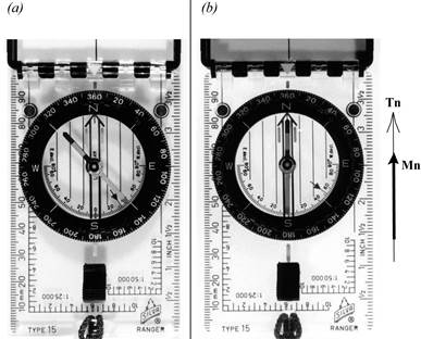
Figure 7.4. Finding true north at 0° declination

Finding 060°

1. Turn the direction ring to align “60” with the white mark near the hinge (Fig. 7.5a).
2. Hold the base of the compass flat and horizontal, with the mirror-end pointing away from you, and turn your body until the compass needle is aligned with the outline arrow, red end toward “N” on the direction ring.

The compass is now aligned along 060°-240°, and you are facing 060°.

Finding 315°

Repeat the directions above, but this time use “315” on the direction ring. (Remember that the white direction marks on the direction ring are in 2° increments.) When you are done, your compass will be aligned along 315°-135°, and you will be facing 315° (Fig. 7.5b).

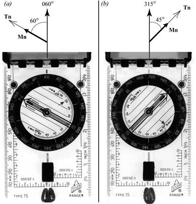
Figure 7.5. Finding 060° and 315° at 0° declination

Case 2: 15° E Declination

1. Turn the brass screw to align the centre mark of the outline arrow with the 15° position on the eastern side of the calibrated base plate (Fig. 7.6a). The eastern side is labelled “E. decl.” You will be turning the outline arrow clockwise from “0”. The compass is now set up to read in terms of true geographic directions for locations with a magnetic declination of 15° E.
2. Repeat the directions from Case 1 for finding true north (Fig. 7.6b) and 060° (Fig. 7.7a). When you are done and facing in the appropriate direction, you will find that your compass needle will be pointing toward magnetic north, slightly to your right.
3. Now find 140° (Fig. 7.7b). When you are done, your compass will be aligned along 140°-320°, and you will be facing 140°.

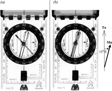
Figure 7.6. Finding true north at 15°E declination

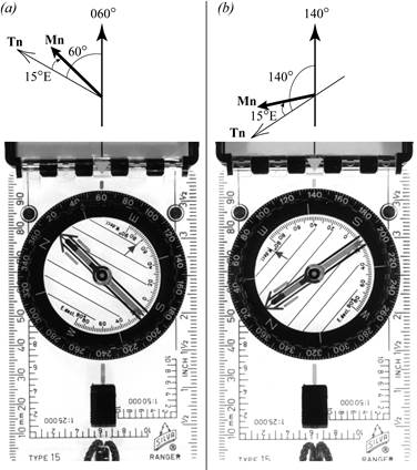
Figure 7.7. Finding 060° and 140° at 15°E declination

Case 3: 20°W Declination

1. Using the brass screw, adjust the outline arrow to the 20° position on the western side of the calibrated base plate (labelled “W. decl.”). Because your skills with the compass are improving, we will try only one example at this declination: 045°.
2. Set the direction ring to 045° and repeat the directions as before. When you are done, the long axis of your compass will be aligned along 045°-225°, and you will be facing 045°. Your compass needle will be pointing slightly to your left (Fig. 7.8).

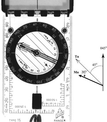
Figure 7.8. Finding 045° at 20°W declination

If by now you find these procedures easy, go on with Case 4, below. If you do not yet feel at ease with your Silva, repeat the three cases above. You might also find it helpful to seek assistance from someone familiar with the use of a compass, such as a member of the armed forces, a pilot, a faculty member of a nearby geology department, or a member of a community scouting organization. A mournful cry of “Does anyone know how to use a compass?” in a public park may also elicit assistance. (Just be prepared to kindly turn down those who offer to find a location for you using the GPS application on their cell phone.)

Case 4: Using Your Local Magnetic Declination

First, set your Silva for the local magnetic declination. You may use Figure 7.2 as a guide, or use the declination (to the nearest degree) of a city listed in Table 7.1. Alternatively, you may determine your local magnetic declination via the online resource.

Preset Directions

Using the previous instructions as a guide, find the following directions: 000°, 020°, 115°, 222°, 293°, and 336°. Remember to point the mirror end of your compass away from you.

Directions to Objects

Identify three objects in widely different directions (houses, cars, trees, etc.) and determine the directions to them as follows:

1. Point the mirror end of the compass toward the object, making sure that the axis of the compass is straight in line between you and the object.
2. Turn the direction ring to align the point of the outline arrow with the red end of the magnetic compass needle.
3. Read the direction off the direction ring, using the white mark at the base of the hinge. If you read the direction ring using the white mark in front of the clip, you will be reading the direction from the object to you (sometimes this is a required procedure).

If you feel comfortable with measuring directions to objects, then carry on with the next section. If not, then select several new objects and continue to practice.

Lesson 3: Measuring Strike and Dip

Strike and Dip Model

For this part of the lab, you will use the strike and dip model included in the lab kit you borrowed from the AU Library. The model consists of two hinged, white, foam-core sheets, and a bundle of eight small sticks with tapered ends.

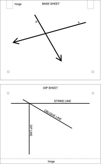
Figure 7.9. Strike and dip model showing the base sheet, dip sheet, and hinge

The base sheet of the model is marked with two long arrows labelled A and B (Fig. 7.9). The other part of the model is the dip sheet. It is marked with a horizontal strike line, a vertical dip line, and an oblique line (Fig. 7.9). Both the base sheet and the dip sheet have holes in the two corners opposite the hinge.

1. Put the model together as shown in Figure 7.10. Use the second-longest set of sticks (approximately 16.5 cm long).
2. Place the model on a non-magnetic surface, such as a wooden table or cardboard box, near the centre of a room or outdoors.
3. Using your Silva compass and the local magnetic declination, find due north.
4. Orient the model so that the arrow A points due north.
5. Anchor the model by placing a heavy non-magnetic object on the base sheet or by taping the base sheet to your working surface.

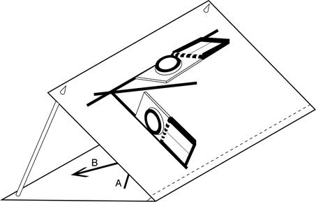
Figure 7.10. How to set up the strike and dip model

How to Measure Strike

Measuring strike is the same as measuring the direction of a horizontal line between you and an object. To measure strike on the model, carry out the following steps:

1. Hold your Silva compass with the base horizontal.
2. Place one edge of the compass along the strike line, as shown in Figure 7.10.
3. Rotate the direction ring until the outline arrow is aligned with the magnetic needle. As you do this, be careful not to nudge the model out of its position.
4. Lift the compass away from the model, and read the direction from the direction ring. You may take the strike reading by using either the white mark by the mirror hinge or the mark beside the clip. For now, record both.

You should have recorded readings of 015° and 195°. An error of ±5° is acceptable. You may use either 015° or 195° as the strike, because they are merely opposite senses of direction. By convention, however, we will use the smaller number. Therefore, we have measured a strike of 015°.

Always record the strike (or trend) as a three-digit number, including the leading 0 or 00 when necessary. This makes it clear to your tutor what you are measuring. It also prevents you from wondering whether the reading you recorded in the field three weeks ago as “50” (at a difficult-to-access site) refers to a strike or a dip (or something unrelated).

How to Measure Dip

To measure dip, it is necessary to first adjust your compass so that it works as an inclinometer. Do this by rotating the direction ring until the “90” on the calibrated base plate is aligned either with the white mark beside the clip or with the white mark beside the mirror hinge.

Previously, you used the scale on the calibrated base plate to indicate magnetic declination, but now you will use it along with the inclinometer arm (the floppy red arrow) to measure vertical angles.

The measurement of dip actually involves two different measurements: the dip angle and the dip direction.

Dip Angle

To measure the dip angle on the model, carry out the following steps:

1. Hold the base of your compass so that the compass is vertical.
2. Place an edge of the compass along the dip line (Fig. 7.10). Place either the mirror end or the cord end down-hill; use whichever end allows the floppy inclinometer arm to rest against the calibrated inclinometer scale (the calibrated base plate).
3. Pivot the compass just barely off the vertical to prevent the inclinometer arm from binding on the base plate of the compass chamber.
4. Without taking the compass off the dip line, read the dip angle indicated on the calibrated inclinometer scale by the inclinometer arm (i.e., read the angle that the little red arrow points to). Note that the scale is marked off in 2° increments. In Figure 7.11, you can see an example of how the inclinometer would look for a dip angle of 60°.

You should have obtained a dip angle of 50° within an error of ±3°. (If the holes in your model are a little worn out, you will obtain a reading slightly less than 50°).

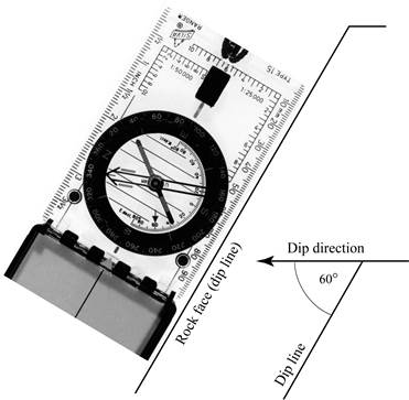
Figure 7.11. View of compass set up as an inclinometer

Always record dip angles as two-digit numbers between 00° and 90°.

To check your technique, confirm that your working surface has a dip of 00° (i.e., check that it is horizontal) and that the dip of your wall is 90°. If either of these measurements is just slightly off, any measurement error may be due to uneven surfaces or shifting structures rather than your ability to use the compass correctly. If your tabletop is not horizontal, correct the dip of your model accordingly, or prop up your table to make it horizontal.

Dip Direction

To measure dip direction, determine the horizontal direction of the dip line in the down-dip direction (Fig. 7.11). This is done by holding your compass over the dip line, with the mirror end pointing in the dip direction, and measuring the dip direction as you would any other direction. For your model, you should get a dip direction of approximately 105°.

The dip of the dip sheet on your model is 50° toward 105°. This is more commonly written as

Dip: 50°/150°

If a geologist records both the dip angle and the precise dip direction as above, then it is unnecessary to also measure and record the strike, because the strike is perpendicular to the dip direction. That is, the strike can be obtained simply by adding 90° to the dip direction.

Lesson 4: Measuring the Orientation of Lines Other than Strike and Dip

The oblique line on the dip sheet of your model is an example of a line other than strike or dip. There are two ways of measuring such lines: pitch (or rake), and plunge and trend.

Pitch

Pitch is measured in a specific plane of interest, as the angle between a line of interest in that plane and a horizontal line on the plane. The downslope direction of the line is also recorded. Pitch is always used in conjunction with strike and dip (or dip and dip direction) of the plane containing the line of interest.

To obtain the pitch of the oblique line on the model requires the following steps:

1. Measure the angle between the strike line and the oblique line with a protractor.
2. Determine the general downslope direction of the line (the quadrant in which the pitch angle was measured.)

You should find that the pitch of the oblique line is 30°NE.

Plunge and Trend

The plunge angle is measured in the vertical plane that contains the line of interest. It is the angle between the line of interest and a horizontal line on the vertical plane. The trend of the line of interest is measured in the same way as that of the dip line.

To measure the plunge of the oblique line on your model, carry out the following steps:

1. Check that your compass is adjusted for measuring inclinations.
2. Hold the base of your compass in a vertical plane.
3. Place an edge of the compass along the oblique line, as you did when measuring dip.
4. Read the plunge angle in the same way as you did the dip angle earlier. You should measure 22°±2°.
5. Next, hold the compass with its base horizontal and directly above the oblique line. Measure the downslope direction of the oblique line in the same way you measured dip direction. You should measure a trend of 036°.

The result of this plunge measurement is 22°/036°. Plunge angles, like dips, are always written as two-digit numbers between 00° and 90°.

Lesson 5: Measuring Small Folds in the Field

In this section you will use the fold model in your lab kit to measure

• the plunge and trend of the hinge line of a fold, and
• the strike and dip of the axial plane of a fold.

Model Assembly

The components of the fold model are shown in Figure 7.12. Carry out the following steps to set up the model as it appears in Figure 7.13:

1. Begin by bending the hinged sheet along its hinge line.
2. Fit the ends of piece C into the slots on the inside of the limbs (A and B) of the hinged sheet. Be sure to match the * and • symbols.

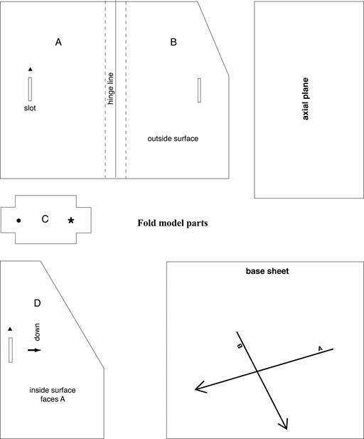
Figure 7.12. Components of the fold model

3. Next, fit sheet D to limb A by matching the slot in D to the end of C that projects through the slot in A. Make sure that the arrow on the inside of D points down, and that the slanted edges of B and D are on the same end of the model. A piece of tape or two on the inside of the model will help to stabilize D.
4. Lay the base plate on a non-magnetic surface with the arrow side up. Using your compass, align the plate so that the arrow A points north.
5. Place the fold model on the base plate with the slanted edge of D along the arrow A, and the hinge line of the model fold pointing down and to the NNW.

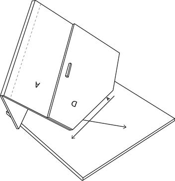
Figure 7.13. Assembled fold model

Measurement of Fold Orientation

We will use two means of measuring fold orientation: a direct method and an indirect method. When you can see the entire fold, as with your model, the direct method is the best to use because it will minimize error. In the field, however, it is not always possible to see the entire fold. The indirect method involves measuring the orientation of the fold limbs only, and then using a stereonet to calculate the orientation of the fold axis and axial plane.

Direct Method

1. Measure and record the plunge angle of the hinge line. Use the same method as you did to measure the dip of the dip line or the plunge of the oblique line on the strike and dip model.
2. Measure and record the trend of the hinge line. This is done the same way as measuring the trend of the dip line or the trend of the oblique line on the strike and dip model.

You should get a result of 23°/340° within an error of 2° for each measurement.

3. Next, measure the strike and dip of the axial plane. You may find it helpful to hold or prop up a stiff, non-magnetic sheet along the model fold's axial plane. You should get a strike and dip of 168°/70°W. A measurement error of up to 5° is acceptable for these numbers.
4. Check your measurements by plotting the plunge and trend of the hinge line and the strike and dip of the axial plane using your stereonet. If all of the data were measured and plotted correctly, the plot of the plunge will lie on the plot of the axial plane. Some measurement error is to be expected, but the error should not result in a gap of greater than 5° between the plots.

Indirect Method

If you examine your model, you will see that the hinge line is the line where the fold limbs intersect. This is true even for folds with round hinge zones. This means that you can determine the plunge of the hinge line from the strikes and dips of the limbs.

1. Measure the strike and dip of each of the model fold's limbs. You should get the following results, within an error of ±5°:

   Western limb: 000°/50°W

   Eastern limb: 160°/vert.

2. On a new overlay, plot the planes of the limbs. Determine the plunge and trend of the point at which the limbs intersect. This value should match the plunge and trend that you measured using the direct method.

   The indirect method may seem familiar, because you used it when you constructed a β-diagram in Lab 6. The only difference is that here you measured the orientations, but in Lab 6 the orientations were provided for you.

If you were to plot the limbs using a π-diagram instead, you could use the bisectrix method to find the strike and dip of the axial plane.

Assignment 7

You should now complete the lab portion of Assignment 7, which you can find in the assignment drop box. Assignment 7 is worth 6% of your final grade (theory portion: 2.5%; lab portion: 3.5%).

After you have completed Assignment 7, please submit this assignment (both theory and lab portions) to your tutor for grading. Please submit your assignment via the appropriate assignment drop box at your online course site. If you are unable to use the assignment drop box, please contact your tutor for an alternative submission method.

After you have completed the final assignment, please send the lab kit back to the AU Library.

Final Exam

If you have not already arranged to write your final exam, please do so at this time. [Please see the online Student Manual for further instructions.] The final examination takes place in two parts: theory (based on material presented in the Study Guide and associated readings and exercises) and application (based on the lab material and associated readings and exercises). The theory portion of the exam includes short-answer and essay-type questions. The lab portion of the exam includes problems similar to those in the Lab portions of your assignments. The theory exam is worth 33% of your final grade, and the lab exam is worth 25%.

You may write both parts of the exam on the same day, or you may opt to write the sections on different days. Each part is invigilated and closed-book. The order in which you write the sections (theory then lab, or lab then theory) is up to you. Because each part of the exam can stand alone, you will need to make separate arrangements for each. This includes making two exam requests (even if you write the exams back-to-back), and if your invigilator requires an exam fee, it may include two exam fees (for which you are responsible). How such fees (if any) are assessed is at the discretion of the invigilation centre. You may find that writing the parts back-to-back is assessed a single fee, while writing each part on a different day is assessed two exam fees. We recommend that you discuss your options and associated fees with your chosen invigilation centre prior to scheduling your exam session(s). There are no exam fees assessed at AU exam centres (Calgary, Edmonton, Athabasca).